本当に売上に貢献している広告は、どの広告か？

売上と広告媒体等との関係性をモデリングし、どの広告媒体が売上にどれほど貢献していたのか分析することができます。

それが、マーケティングミックスモデリング（MMM：Marketing Mix Modeling）です。

前回と前々回、アドストック（Ad Stock）を考慮した線形回帰モデルのお話しをしました。

以下は、前々回の記事です。

Pythonによるマーケティングミックスモデリング（MMM：Marketing Mix Modeling）超入門 その2アドストック（Ad Stock）を考慮した線形回帰モデル

以下は、前回の記事です。

Pythonによるマーケティングミックスモデリング（MMM：Marketing Mix Modeling）超入門 その3ちょっと複雑なアドストック（Ad Stock）を考慮した線形回帰モデル

ちなみに、アドストック（Ad Stock）を考慮するとは、飽和効果（収穫逓減）とキャリーオーバー（Carryover）効果を考慮するということです。

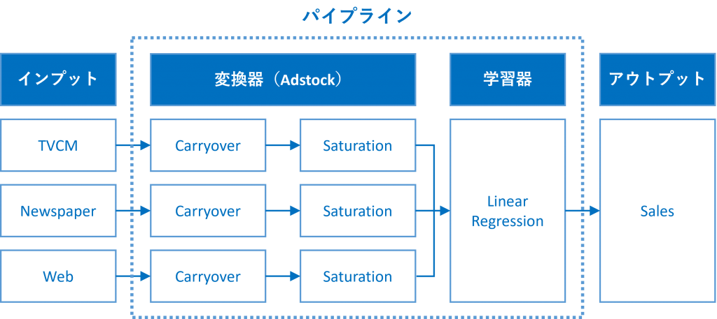
具体的には、Pythonのscikit-learn（sklearn）のパイプラインを、以下のように構築しました。

その中で、幾つかのアドストック（Ad Stock）を表現するモデル（具体的には、関数）を紹介しました。

どのような関数の組み合わせでアドストック（Ad Stock）を表現するがいいのでしょうか？

ということで、今回は「最適なアドストック（Ad Stock）を探索しモデル構築」というお話しをします。

利用するデータセット（前回と同じ）

今回利用するデータセットの変数です。

• Week：週
• Sales：売上
• TVCM：TV CMのコスト
• Newspaper：新聞の折り込みチラシのコスト
• Web：Web広告のコスト

以下からダウンロードできます。

MMM.csv
https://www.salesanalytics.co.jp/4zdt

アドストック（Ad Stock）

今回は、以下の関数の中から最適な組み合わせを探し、アドストック（Ad Stock）を表現し、モデル構築したいと思います。

• キャリーオーバー効果モデル
  • 定率減少型キャリーオーバー効果モデル　※ピークが広告などの投入時（simple_Carryover）
  • ピーク可変型キャリーオーバー効果モデル（peak_Carryover）
• 飽和モデル
  • 指数型飽和モデル（exp_Saturation）
  • ロジスティック型飽和モデル（logit_Saturation）
  • ゴンペルツ型飽和モデル（gom_Saturation）

具体的には、2種類のキャリーオーバー効果モデルから関数を1つ、3種類の飽和モデルから関数を1つ選びます。

　2つのキャリーオーバー効果モデル

以下は、ピークが広告などの投入時で徐々に低減する「定率減少型キャリーオーバー効果モデル」です。当期にピークが来ています。

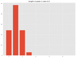
以下は、ピークが広告などの投入時に限らない「ピーク可変型キャリーオーバー効果モデル」です。次期にピークが来ています。

　3つの飽和モデル

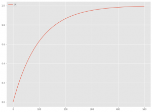
以下は、「指数型飽和モデル」です。

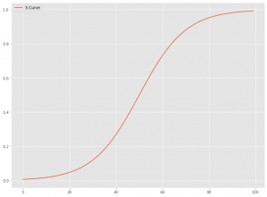
以下は、「S字曲線型飽和モデル」です。S字曲線型飽和モデルには幾つかありますが、今回は「ロジスティック型飽和モデル」と「ゴンペルツ型飽和モデル」を使います。

ライブラリーやデータセットなどの読み込み

先ずは、必要なライブラリーとデータセットを読み込みます。前回までと同じです。

　必要なライブラリーの読み込み

必要なライブラリーを読み込みます。

以下、コードです。

import numpy as np
import pandas as pd

from scipy.signal import convolve2d

from sklearn.base import BaseEstimator, TransformerMixin
from sklearn.compose import ColumnTransformer
from sklearn.pipeline import Pipeline
from sklearn.model_selection import cross_val_score, TimeSeriesSplit
from sklearn import set_config

from sklearn.linear_model import LinearRegression

import optuna
from optuna.integration import OptunaSearchCV
from optuna.distributions import UniformDistribution, IntUniformDistribution, CategoricalDistribution

import matplotlib.pyplot as plt
plt.style.use('ggplot') #グラフスタイル
plt.rcParams['figure.figsize'] = [12, 9] # グラフサイズ

#指数表記しない設定
np.set_printoptions(precision=3,suppress=True)
pd.options.display.float_format = '{:.3f}'.format

　データセット（前回と同じ）の読み込み

前回と同じデータセットを読み込みます。

以下、コードです。

# データセット読み込み
url = 'https://www.salesanalytics.co.jp/4zdt'
df = pd.read_csv(url,
                 parse_dates=['Week'],
                 index_col='Week'
                )

# データ確認
print(df.info()) #変数の情報
print(df.head()) #データの一部

# 説明変数Xと目的変数yに分解
X = df.drop(columns=['Sales'])
y = df['Sales']

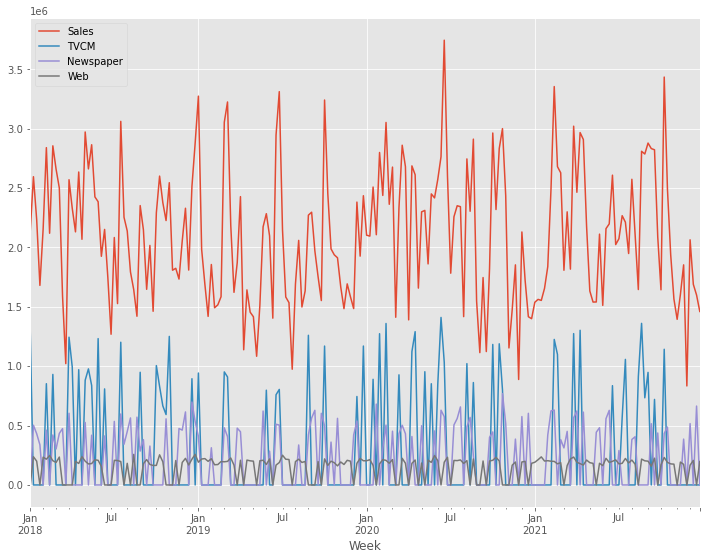
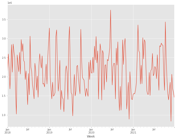
# グラフ化
y.plot()
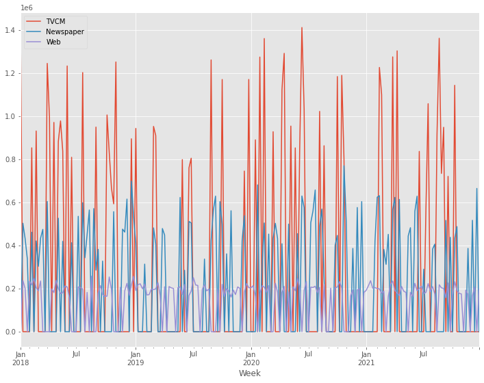
X.plot()

以下、実行結果です。

アドストックを考慮しない線形回帰モデル

アドストックを考慮しない線形回帰モデルを構築し、どの程度の精度を持ったものだったのかを見てみます。

ちなみに、前回と同じものです。

線形回帰モデルのインスタンスを作ります。

以下、コードです。

# 線形回帰モデルのインスタンス
lr = LinearRegression()

線形回帰モデルが、どの程度の予測精度を持ったモデルになるのかを確かめるために、時系列のCV（クロスバリデーション）を実施します。今回は、デフォルトの5分割のCVです。

以下、コードです。

# クロスバリデーションで精度検証（R2）
np.mean(cross_val_score(lr, 
                        X, y, 
                        cv=TimeSeriesSplit()
                       )
       )

以下、実行結果です。

全データでモデルを構築し、予測精度（$R^2$）を見てみます。

以下、コードです。

# 全データで精度検証（R2）
lr.fit(X, y)
lr.score(X, y)

以下、実行結果です。

アドストックを考慮した線形回帰モデル
（Optunaでハイパーパラメータチューニング）

Optunaで最適な飽和モデルとキャリーオーバー効果モデルの組み合わせを探しつつ、それぞれのモデルのハイパーパラメータチューニングをします。

　アドストックを表現する関数の設定

個々の飽和モデルとキャリーオーバー効果モデルの関数を定義し、その関数の変換器クラスを構築します。

　　飽和モデル

以下の3つの飽和モデルの関数を定義し、その関数の変換器クラスを構築します。

• 指数型飽和モデル（exp_Saturation）
• ロジスティック型飽和モデル（logit_Saturation）
• ゴンペルツ型飽和モデル（gom_Saturation）

先ず、飽和モデルの関数をそれぞれ定義します。

以下、指数型飽和モデルの関数です。

# 指数型飽和モデル（exp_Saturation）
def exp_Saturation(X,a):
    return 1 - np.exp(-a*X)

以下、ロジスティック型飽和モデルの関数です。

# ロジスティック型飽和モデル（logit_Saturation）
def logit_Saturation(X,K,b,c,m):
    return K/(1+b*np.exp(-c*(X-m)))

以下、ゴンペルツ型飽和モデルの関数です。

# ゴンペルツ型飽和モデル（gom_Saturation）
def gom_Saturation(X,K,b,c,m):
    return K*(b**np.exp(-c*(X-m)))

次に、定義した関数を使い飽和モデルの変換器クラスを構築します。

以下、指数型飽和モデルの変換器です。

# 指数型飽和モデル（exp_Saturation）
class pipe_exp_Saturation(BaseEstimator, TransformerMixin):
    
    # 初期化
    def __init__(self,a=1.0):
        self.a = a
    
    # 学習
    def fit(self, X, y=None):
        return self
    
    # 処理（入力→出力）
    def transform(self, X):
        X_ = exp_Saturation(X,
                            self.a
                           ).reshape(-1,1)
        return X_

以下、ロジスティック型飽和モデルの変換器です。

# ロジスティック型飽和モデル（logit_Saturation）
class pipe_logit_Saturation(BaseEstimator, TransformerMixin):
    
    # 初期化
    def __init__(self,K=1.0,m=100.0,b=1.0, c=0.1):
        self.K = K
        self.m = m
        self.b = b
        self.c = c
    
    # 学習
    def fit(self, X, y=None):
        return self
    
    # 処理（入力→出力）
    def transform(self, X):
        X_ = logit_Saturation(X,
                              self.K, 
                              self.b, 
                              self.c, 
                              self.m
                             ).reshape(-1,1)
        return X_

以下、ゴンペルツ型飽和モデルの変換器です。

# ゴンペルツ型飽和モデル（gom_Saturation）
class pipe_gom_Saturation(BaseEstimator, TransformerMixin):
    
    # 初期化
    def __init__(self,K=1.0,m=100.0,b=1.0,c=0.1):
        self.K = K
        self.m = m
        self.b = b
        self.c = c
    
    # 学習
    def fit(self, X, y=None):
        return self
    
    # 処理（入力→出力）
    def transform(self, X):
        X_ = gom_Saturation(X,
                            self.K, 
                            self.b, 
                            self.c, 
                            self.m
                           ).reshape(-1,1)
        return X_

　　キャリーオーバー効果モデル

以下の2つのキャリーオーバー効果モデルの関数を定義し、その関数の変換器クラスを構築します。

• 定率減少型キャリーオーバー効果モデル　※ピークが広告などの投入時（simple_Carryover）
• ピーク可変型キャリーオーバー効果モデル（peak_Carryover）

先ず、キャリーオーバー効果モデルの関数を定義します。

以下、定率減少型キャリーオーバー効果モデルの関数です。

# 定率減少型キャリーオーバー効果モデル　※ピークが広告などの投入時（simple_Carryover）
def simple_Carryover(X: np.ndarray, rate, length):
    
    filter = (
        rate ** np.arange(length + 1)
    ).reshape(-1, 1) 
    
    convolution = convolve2d(X, filter)
    
    if length > 0 : convolution = convolution[: -length]
        
    return convolution[:,0]

以下、ピーク可変型キャリーオーバー効果モデルの関数です。

# ピーク可変型キャリーオーバー効果モデル（peak_Carryover）
def peak_Carryover(X: np.ndarray, length, peak, rate):
    X = np.append(np.zeros(length-1), X)
    
    Ws = np.zeros(length)
    
    for l in range(length):
        W = rate**((l-peak)**2)
        Ws[length-1-l] = W
    
    carryover_X = []
    
    for i in range(length-1, len(X)):
        X_array = X[i-length+1:i+1]
        Xi = sum(X_array * Ws)/sum(Ws)
        carryover_X.append(Xi)
        
    return np.array(carryover_X)

次に、定義した関数を使いキャリーオーバー効果モデルの変換器クラスを構築します。

以下、定率減少型キャリーオーバー効果モデルの変換器です。

# 定率減少型キャリーオーバー効果モデル　※ピークが広告など投入時（simple_Carryover）
class pipe_simple_Carryover(BaseEstimator, TransformerMixin):

    # 初期化
    def __init__(self,length=4,rate=0.5):
        self.length = length
        self.rate = rate
        
    # 学習        
    def fit(self, X, y=None):
        return self

    # 処理（入力→出力）
    def transform(self, X):
        X_ = simple_Carryover(X, 
                              self.rate, 
                              self.length
                             )
        return X_

以下、ピーク可変型キャリーオーバー効果モデルの変換器です。

# Pipeline用変換器（キャリーオーバー効果モデル）
class pipe_peak_Carryover(BaseEstimator, TransformerMixin):

    # 初期化
    def __init__(self,length=4,peak=1,rate=0.5):
        self.length = length
        self.peak = peak
        self.rate = rate
        
    # 学習        
    def fit(self, X, y=None):
        return self

    # 処理（入力→出力）
    def transform(self, X):
        X_ = peak_Carryover(X, 
                            self.length, 
                            self.peak, 
                            self.rate
                           ) 
        return X_

　パイパーパラメータ探索の実施

Optunaを使い関数の組み合わせと、それぞれの関数の最適なパイパーパラメータを探索します。

Optunaを使ったハイパーパラメータチューニングに関しては、以下の一連の記事を参考にして頂ければと思います。

先ずは、Optunaで利用する目的関数を定義します。

以下、コードです。

# 目的関数の設定
def objective(trial):
    
    #TVCM
    
    ##TVCM Adstock func
    
    TVCM_Saturation_func = trial.suggest_categorical(
        "TVCM_Saturation_func",
        ["exp", "logit","gom"]
    )
    
    TVCM_Carryover_func = trial.suggest_categorical(
        "TVCM_Carryover_func",
        ["simple", "peak"]
    )
    
    ##TVCM_Saturation
    
    if TVCM_Saturation_func == 'exp':
        
        TVCM_a = trial.suggest_float(
            "TVCM_a", 
            0, 0.01
        )
        
        TVCM_Saturation = pipe_exp_Saturation(a=TVCM_a)
        
    elif TVCM_Saturation_func == 'logit':
        
        TVCM_K = trial.suggest_float(
            "TVCM_K", 
            np.min(X.TVCM), np.max(X.TVCM)*2
        )
        TVCM_m = trial.suggest_float(
            "TVCM_m",
            np.min(X.TVCM), np.max(X.TVCM)
        )
        TVCM_b = trial.suggest_float(
            "TVCM_b",
            0, 10
        )
        TVCM_c = trial.suggest_float(
            "TVCM_c",
            0, 1
        )
        
        TVCM_Saturation = pipe_logit_Saturation(
            K=TVCM_K,
            m=TVCM_m,
            b=TVCM_b,
            c=TVCM_c
        )
        
    else:
        
        TVCM_K = trial.suggest_float(
            "TVCM_K", 
            np.min(X.TVCM), 
            np.max(X.TVCM)*2
        )
        TVCM_m = trial.suggest_float(
            "TVCM_m", 
            np.min(X.TVCM), 
            np.max(X.TVCM)
        )
        TVCM_b = trial.suggest_float(
            "TVCM_b", 
            0, 1
        )
        TVCM_c = trial.suggest_float(
            "TVCM_c", 
            0, 1
        )     
        
        TVCM_Saturation = pipe_gom_Saturation(
            K=TVCM_K,
            m=TVCM_m,
            b=TVCM_b,
            c=TVCM_c
        )
        
    ##TVCM Carryover
    
    if TVCM_Carryover_func == 'simple':
        
        TVCM_rate = trial.suggest_float(
            "TVCM_rate", 
            0,1
        )
        TVCM_length = trial.suggest_int(
            "TVCM_length", 
            0,6
        )
        
        TVCM_Carryover = pipe_simple_Carryover(
            length=TVCM_length,
            rate=TVCM_rate
        )
        
    else:
        
        TVCM_rate = trial.suggest_float(
            "TVCM_rate", 
            0, 1
        )
        TVCM_length = trial.suggest_int(
            "TVCM_length",
            1,7
        )
        TVCM_peak = trial.suggest_int(
            "TVCM_peak",
            0,2
        )
        
        TVCM_Carryover = pipe_peak_Carryover(
            length=TVCM_length, 
            rate=TVCM_rate,
            peak=TVCM_peak
        )   

    #Newspaper
    
    ##Newspaper Adstock func
    
    Newspaper_Saturation_func = trial.suggest_categorical(
        "Newspaper_Saturation_func",
        ["exp", "logit","gom"]
    )
    
    Newspaper_Carryover_func = trial.suggest_categorical(
        "Newspaper_Carryover_func",
        ["simple", "peak"]
    )
    
    ##Newspaper_Saturation
    
    if Newspaper_Saturation_func == 'exp':
        
        Newspaper_a = trial.suggest_float(
            "Newspaper_a", 
            0, 0.01
        )
        
        Newspaper_Saturation = pipe_exp_Saturation(a=Newspaper_a)
        
    elif Newspaper_Saturation_func == 'logit':
        
        Newspaper_K = trial.suggest_float(
            "Newspaper_K",
            np.min(X.Newspaper), np.max(X.Newspaper)*2
        )
        Newspaper_m = trial.suggest_float(
            "Newspaper_m", 
            np.min(X.Newspaper), np.max(X.Newspaper)
        )
        Newspaper_b = trial.suggest_float(
            "Newspaper_b", 
            0, 10
        )
        Newspaper_c = trial.suggest_float(
            "Newspaper_c", 
            0, 1
        )
        
        Newspaper_Saturation = pipe_logit_Saturation(
            K=Newspaper_K,
            m=Newspaper_m,
            b=Newspaper_b,
            c=Newspaper_c
        )
        
    else:
        
        Newspaper_K = trial.suggest_float(
            "Newspaper_K", 
            np.min(X.Newspaper), np.max(X.Newspaper)*2
        )
        Newspaper_m = trial.suggest_float(
            "Newspaper_m", 
            np.min(X.Newspaper), np.max(X.Newspaper)
        )
        Newspaper_b = trial.suggest_float(
            "Newspaper_b", 
            0, 1
        )
        Newspaper_c = trial.suggest_float(
            "Newspaper_c", 
            0, 1
        )     
        
        Newspaper_Saturation = pipe_gom_Saturation(
            K=Newspaper_K,
            m=Newspaper_m,
            b=Newspaper_b,
            c=Newspaper_c
        )
        
    ##Newspaper Carryover
    
    if Newspaper_Carryover_func == 'simple':
        
        Newspaper_rate = trial.suggest_float(
            "Newspaper_rate", 
            0,1
        )
        Newspaper_length = trial.suggest_int(
            "Newspaper_length", 
            0,6
        )
        
        Newspaper_Carryover = pipe_simple_Carryover(
            length=Newspaper_length,
            rate=Newspaper_rate
        )
        
    else:
        
        Newspaper_rate = trial.suggest_float(
            "Newspaper_rate", 
            0, 1
        )
        Newspaper_length = trial.suggest_int(
            "Newspaper_length",
            1,7
        )
        Newspaper_peak = trial.suggest_int(
            "Newspaper_peak",
            0,2
        )
        
        Newspaper_Carryover = pipe_peak_Carryover(
            length=Newspaper_length,
            rate=Newspaper_rate,
            peak=Newspaper_peak
        )
            
    #Web
    
    ##Web Adstock func
    
    Web_Saturation_func = trial.suggest_categorical(
        "Web_Saturation_func",
        ["exp", "logit","gom"]
    )
    
    Web_Carryover_func = trial.suggest_categorical(
        "Web_Carryover_func",
        ["simple", "peak"]
    )
    
    ##Web_Saturation
    
    if Web_Saturation_func == 'exp':
        
        Web_a = trial.suggest_float(
            "Web_a", 
            0, 0.01
        )
        
        Web_Saturation = pipe_exp_Saturation(a=Web_a)
        
    elif Web_Saturation_func == 'logit':
        
        Web_K = trial.suggest_float(
            "Web_K", 
            np.min(X.Web), np.max(X.Web)*2
        )
        Web_m = trial.suggest_float(
            "Web_m", 
            np.min(X.Web), np.max(X.Web)
        )
        Web_b = trial.suggest_float(
            "Web_b", 
            0, 10
        )
        Web_c = trial.suggest_float(
            "Web_c", 
            0, 1
        )
        
        Web_Saturation = pipe_logit_Saturation(
            K=Web_K,
            m=Web_m,
            b=Web_b,
            c=Web_c
        )
        
    else:
        
        Web_K = trial.suggest_float(
            "Web_K", 
            np.min(X.Web), np.max(X.Web)*2
        )
        Web_m = trial.suggest_float(
            "Web_m", 
            np.min(X.Web), np.max(X.Web)
        )
        Web_b = trial.suggest_float(
            "Web_b", 
            0, 1
        )
        Web_c = trial.suggest_float(
            "Web_c", 
            0, 1
        )     
        
        Web_Saturation = pipe_gom_Saturation(
            K=Web_K,
            m=Web_m,
            b=Web_b,
            c=Web_c
        )
        
    ##Web Carryover
    
    if Web_Carryover_func == 'simple':
        
        Web_rate = trial.suggest_float(
            "Web_rate", 
            0,1
        )
        Web_length = trial.suggest_int(
            "Web_length", 
            0,6
        )
        
        Web_Carryover = pipe_simple_Carryover(
            length=Web_length,
            rate=Web_rate
        )
        
    else:
        
        Web_rate = trial.suggest_float(
            "Web_rate", 
            0, 1
        )
        Web_length = trial.suggest_int(
            "Web_length",
            1,7
        )
        Web_peak = trial.suggest_int(
            "Web_peak",
            0,2
        )
        
        Web_Carryover = pipe_peak_Carryover(
            length=Web_length,
            rate=Web_rate,
            peak=Web_peak
        )   
    
    # パイプライン化
    
    ## 変換器（Adstock）
    adstock = ColumnTransformer(
        [
         ('TVCM_pipe', Pipeline([
             ('TVCM_carryover', TVCM_Carryover),
             ('TVCM_saturation', TVCM_Saturation)
         ]), ['TVCM']),
         ('Newspaper_pipe', Pipeline([
             ('Newspaper_carryover', Newspaper_Carryover),
             ('Newspaper_saturation', Newspaper_Saturation)
         ]), ['Newspaper']),
         ('Web_pipe', Pipeline([
             ('Web_carryover', Web_Carryover),
             ('Web_saturation', Web_Saturation)
         ]), ['Web']),
        ],
        remainder='passthrough'
    )

    ## 説明変数の変換（adstock）→線形回帰モデル（regression）
    MMM_pipe = Pipeline([
        ('adstock', adstock),
        ('regression', LinearRegression())
    ])
        
    #CVによる評価
    score = cross_val_score(
        MMM_pipe,
        X,
        y,
        cv=TimeSeriesSplit()
    )
    accuracy = score.mean()
    return accuracy

分かりやすくするため、ベタに長めのコードにしています。頭の方から説明すると、飽和モデルとキャリーオーバー効果モデルの関数の選択があり、その後に選択された関数に応じてIf文でそれぞれの変換器を選択しています。それを、TVCM、Newspaper、Webの順番に冗長に繰り返しています。そして、選択した変換器を使いパイプラインを構築しCV（クロスバリデーション）評価をしています。

この目的関数に対し最適化を実行することで、最適な関数の組み合わせとそれぞれのハイパーパラメータを探索します。

以下、コードです。実行時間が長く終了しない場合には、「n_trials」の数字を小さくして下さい。

# 目的関数の最適化を実行する
study = optuna.create_study(direction="maximize")
study.optimize(objective,
               n_trials=5000,
               show_progress_bar=True)

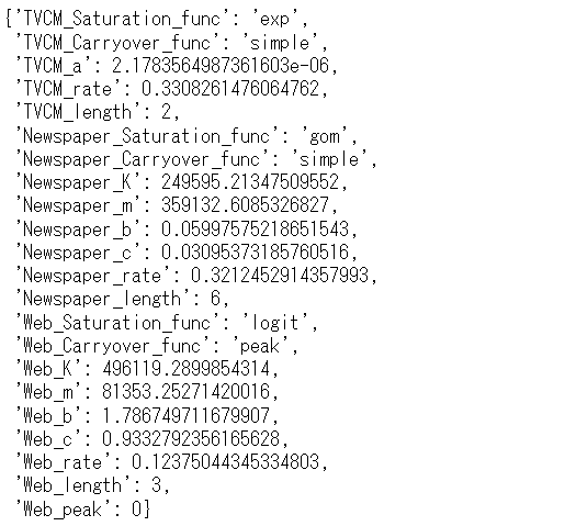
探索が終了したら、結果を見てみます。

以下、コードです。

# 探索結果
study.best_params

以下、実行結果です。

　最適なハイパーパラメータでパイプラインを学習

求めた最適なハイパーパラメータでモデル構築し精度検証します。

具体的には、先ずパイプラインの定義をします。次に、そのパイプラインに最適なハイパーパラメータを設定します。そのパイプラインを使い、精度検証をします。

　　パイプライン構築

パイプライン用の、飽和モデルとキャリーオーバー効果の2つの変換器クラスを定義します。

以下、コードです。

# Pipeline用変換器

## 飽和モデル

class Saturation(BaseEstimator, TransformerMixin):
    
    # 初期化
    def __init__(self,func='exp',a=1.0,K=1.0,m=100.0,b=1.0, c=0.1):
        self.func = func
        self.a = a
        self.K = K
        self.m = m
        self.b = b
        self.c = c
    
    # 学習
    def fit(self, X, y=None):
        return self
    
    # 処理（入力→出力）
    def transform(self, X):
        if self.func == 'exp':
            X_ = exp_Saturation(X,
                                self.a
                               ).reshape(-1,1)
        elif self.func == "logit":
            X_ = logit_Saturation(X,
                                  self.K, 
                                  self.b,
                                  self.c, 
                                  self.m
                                 ).reshape(-1,1)
        else:
            X_ = gom_Saturation(X,
                                self.K, 
                                self.b, 
                                self.c, 
                                self.m
                               ).reshape(-1,1)
        return X_
    
## キャリーオーバー効果モデル

class Carryover(BaseEstimator, TransformerMixin):

    # 初期化
    def __init__(self,func='simple',length=4, peak=1, rate=0.5):
        self.func = func
        self.length = length
        self.peak = peak
        self.rate = rate
        
    # 学習        
    def fit(self, X, y=None):
        return self

    # 処理（入力→出力）
    def transform(self, X):
        if self.func == 'peak':
            X_ = peak_Carryover(X, 
                                self.length, 
                                self.peak, 
                                self.rate)  
        else:
            X_ = simple_Carryover(X, 
                                  self.rate, 
                                  self.length)
            
        return X_

この2つの変換器でアドストック（Ad Stock）を表現します。これらの変換器と学習器（線形回帰モデル）をつなげたパイプラインを構築します。

以下、コードです。

# Pipelineの設定

## 説明変数の変換部分（adstock）の定義
adstock = ColumnTransformer(
    [
     ('TVCM_pipe', Pipeline([
                           ('carryover', Carryover()),
                           ('saturation', Saturation())
     ]), ['TVCM']),
     ('Newspaper_pipe', Pipeline([
                           ('carryover', Carryover()),
                           ('saturation', Saturation())
     ]), ['Newspaper']),
     ('Web_pipe', Pipeline([
                           ('carryover', Carryover()),
                           ('saturation', Saturation())
     ]), ['Web']),
    ],
    remainder='passthrough'
)

## 説明変数の変換（adstock）→線形回帰モデル（regression）
MMM_pipe = Pipeline([
    ('adstock', adstock),
    ('regression', LinearRegression())
])

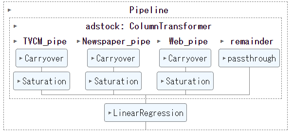
## パイプラインの確認
set_config(display='diagram')   
MMM_pipe

以下、実行結果です。

このパイプラインに、先程求めた最適なハイパーパラメータを設定します。

以下、コードです。

# パイプラインのハイパーパラメータの設定
best_params={
 'adstock__TVCM_pipe__carryover__func': 
    study.best_params.get('TVCM_Carryover_func'),
 'adstock__TVCM_pipe__carryover__length': 
    study.best_params.get('TVCM_length'),
 'adstock__TVCM_pipe__carryover__peak': 
    study.best_params.get('TVCM_peak'),
 'adstock__TVCM_pipe__carryover__rate': 
    study.best_params.get('TVCM_rate'),
 'adstock__TVCM_pipe__saturation__func': 
    study.best_params.get('TVCM_Saturation_func'),
 'adstock__TVCM_pipe__saturation__a': 
    study.best_params.get('TVCM_a'),
 'adstock__TVCM_pipe__saturation__K': 
    study.best_params.get('TVCM_K'),
 'adstock__TVCM_pipe__saturation__m': 
    study.best_params.get('TVCM_m'),
 'adstock__TVCM_pipe__saturation__b': 
    study.best_params.get('TVCM_b'),
 'adstock__TVCM_pipe__saturation__c': 
    study.best_params.get('TVCM_c'),
 'adstock__Newspaper_pipe__carryover__func': 
    study.best_params.get('Newspaper_Carryover_func'),
 'adstock__Newspaper_pipe__carryover__length': 
    study.best_params.get('Newspaper_length'),
 'adstock__Newspaper_pipe__carryover__peak': 
    study.best_params.get('Newspaper_peak'),
 'adstock__Newspaper_pipe__carryover__rate': 
    study.best_params.get('Newspaper_rate'),
 'adstock__Newspaper_pipe__saturation__func': 
    study.best_params.get('Newspaper_Saturation_func'),
 'adstock__Newspaper_pipe__saturation__a': 
    study.best_params.get('Newspaper_a'),
 'adstock__Newspaper_pipe__saturation__K': 
    study.best_params.get('Newspaper_K'),
 'adstock__Newspaper_pipe__saturation__m': 
    study.best_params.get('Newspaper_m'),
 'adstock__Newspaper_pipe__saturation__b': 
    study.best_params.get('Newspaper_b'),
 'adstock__Newspaper_pipe__saturation__c': 
    study.best_params.get('Newspaper_c'),
 'adstock__Web_pipe__carryover__func':
    study.best_params.get('Web_Carryover_func'),
 'adstock__Web_pipe__carryover__length': 
    study.best_params.get('Web_length'),
 'adstock__Web_pipe__carryover__peak': 
    study.best_params.get('Web_peak'),
 'adstock__Web_pipe__carryover__rate': 
    study.best_params.get('Web_rate'),
 'adstock__Web_pipe__saturation__func': 
    study.best_params.get('Web_Saturation_func'),
 'adstock__Web_pipe__saturation__a': 
    study.best_params.get('Web_a'),
 'adstock__Web_pipe__saturation__K': 
    study.best_params.get('Web_K'),
 'adstock__Web_pipe__saturation__m': 
    study.best_params.get('Web_m'),
 'adstock__Web_pipe__saturation__b': 
    study.best_params.get('Web_b'),
 'adstock__Web_pipe__saturation__c': 
    study.best_params.get('Web_c'),
}

　　精度検証

パイプラインのインスタンスを作ります。

以下、コードです。

# パイプラインのインスタンス
MMM_pipe_best = MMM_pipe.set_params(**best_params)

線形回帰モデルが、どの程度の予測精度を持ったモデルになるのかを確かめるために、時系列のCV（クロスバリデーション）を実施します。今回は、デフォルトの5分割のCVです。

以下、コードです。

# クロスバリデーションで精度検証（R2）
np.mean(cross_val_score(MMM_pipe_best, 
                        X, y, 
                        cv=TimeSeriesSplit()
                       )
       )

以下、実行結果です。

全データでモデルを構築し、予測精度（$R^2$）を見てみます。

以下、コードです。

# 全データで精度検証（R2）
MMM_pipe_best.fit(X, y)
MMM_pipe_best.score(X, y)

以下、実行結果です。

アドストックを考慮しない線形回帰モデルに比べ、以下のように（$R^2$）が変化しました。前回と前々回と比較しても、最も良い値がでています。

• CVの$R^2$の平均値：0.70→0.85
• 全データ利用した場合の$R^2$：0.74→0.87

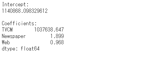
どのような線形回帰モデルなのか（切片と回帰係数）を見てみます。

以下、コードです。

# 線形回帰モデルの切片と回帰係数
intercept = MMM_pipe_best.named_steps['regression'].intercept_ #切片
coef = MMM_pipe_best.named_steps['regression'].coef_ #回帰係数

# 回帰係数をデータフレーム化
weights = pd.Series(
    coef,
    index=X.columns
)

# 結果出力（切片と係数）
print('Intercept:\n', intercept, sep='')
print()
print('Coefficients:\n',weights, sep='')

以下、実行結果です。

　売上貢献度の算出

学習し構築したパイプラインの変換器（adstock）を抽出します。

以下、コードです。

# Piplineの変換器（adstock）を抽出
adstock = MMM_pipe_best.named_steps['adstock']

説明変数を変換し、学習データのインプットデータを作ります。

以下、コードです。

# 説明変数Xの変換
X_trans = pd.DataFrame(adstock.transform(X),
                       index=X.
                       index,columns=X.columns)

先程求めた線形回帰式を使い、売上貢献度（補正前）を計算します。

以下、コードです。

# 貢献度（補正前）
unadj_contribution = X_trans.mul(weights) #Xと係数を乗算
unadj_contribution = unadj_contribution.assign(Base=intercept) #切片の追加

unadj_contribution.head() #確認

以下、実行結果です。

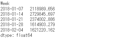
週ごとに各媒体の売上貢献度を合計すると、売上の予測値になります。

以下、コードです。

# 貢献度の合計（yの予測値）
y_pred = unadj_contribution.sum(axis=1)

y_pred.head() #確認

以下、実行結果です。

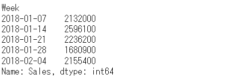
元の売上の実測値を見てみます。

以下、コードです。

y.head() #確認

以下、実行結果です。

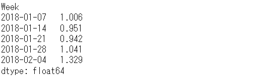
予測値と実測値が乖離していることが分かります。この乖離をなくすために、補正係数（correction factor）を計算し、売上貢献度を補正します。

補正係数を計算します。

以下、コードです。

# 補正係数
correction_factor = y.div(y_pred, axis=0)

correction_factor.head() #確認

以下、実行結果です。

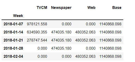
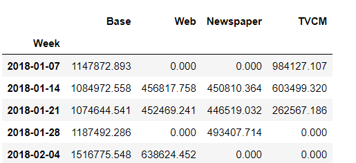
この補正係数を使い、売上貢献度を補正します。

以下、コードです。

# 貢献度（補正後）
adj_contribution = (unadj_contribution
                    .mul(correction_factor, axis=0)
                   ) 

# 順番の変更
adj_contribution = adj_contribution[['Base', 'Web', 'Newspaper', 'TVCM']]

#確認
adj_contribution.head()

以下、実行結果です。

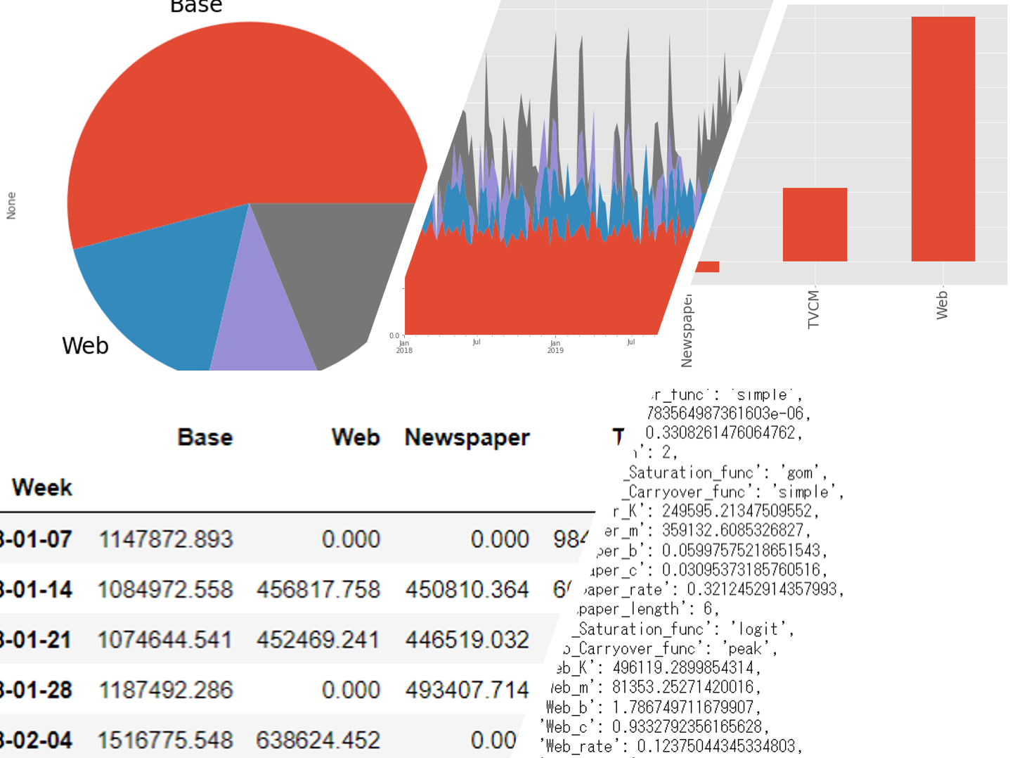
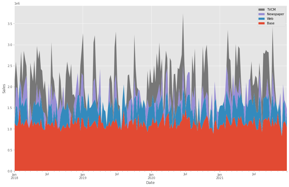
週×媒体別の売上貢献度が求められたので、積み上げグラフを作成し、どのような状況になっているのかを確認してみます。

以下、コードです。

# グラフ化
ax = (adj_contribution
      .plot.area(
          figsize=(16, 10),
          linewidth=0,
          ylabel='Sales',
          xlabel='Date')
     )

handles, labels = ax.get_legend_handles_labels()
ax.legend(handles[::-1], labels[::-1])

以下、実行結果です。

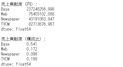
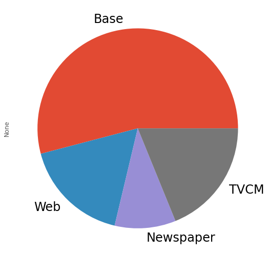
媒体別に全ての週の売上貢献度を合計し、媒体別の売上貢献度（円と構成比％）と、そのグラフを作り、何がどれほど売上に貢献したのかを見てみます。

以下、コードです。

# 媒体別の貢献度の合計
contribution_sum = adj_contribution.sum(axis=0)

#集計結果
print('売上貢献度（円）:\n', 
      contribution_sum, 
      sep=''
     )
print()
print('売上貢献度（構成比）:\n', 
      contribution_sum/contribution_sum.sum(), 
      sep=''
     )

#グラフ化
contribution_sum.plot.pie(fontsize=24)

以下、実行結果です。

費用対効果を見てみます。今回は媒体別にROIを計算します。

先ず、媒体別のコストを集計します。

以下、コードです。

# 各媒体のコストの合計
cost_sum = X.sum(axis=0)

cost_sum #確認

以下、実行結果です。

先程求めた売上貢献度を使い、媒体別のROIを計算しグラフ化します。

以下、コードです。

# 各媒体のROIの計算
ROI = (contribution_sum.drop('Base', axis=0) - cost_sum)/cost_sum

#確認
print('ROI:\n', ROI, sep='')

# グラフ化
ROI.plot.bar(fontsize=24)

以下、実行結果です。

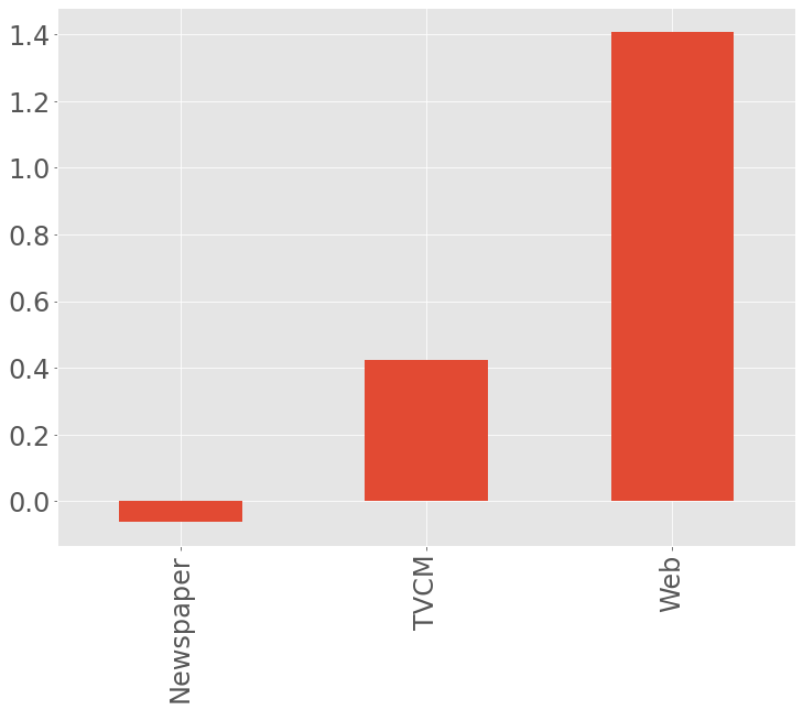
ROIは、値が大きいほど良く、少なくとも0以上である必要があります。

TVCMは0以上なのはTVCMとWebです。Webが非常にいいということが分かります。一方、Newspaperは0未満なので、少なくとも止めたほうが良さそうです。

まとめ

今回は、「最適なアドストック（Ad Stock）を探索しモデル構築」についてお話ししました。

広告などのマーケティング変数は、お互いに強い相関を示すことがあります。なぜならば、同じ時期にキャンペーンという名目で広告などを投入したりするからです。

そのことによって、マルチコという線形回帰モデルにとってやっかいな現象が起こることがあります。

では、どうすればいいのか？

解決策の1つとして、正則化項付き線形回帰モデルというものがあります。俗にいう、Ridge回帰などです。

次回は、「Ridge回帰モデルでマーケティングミックスモデリング」というお話しをします。

Pythonによるマーケティングミックスモデリング（MMM：Marketing Mix Modeling）超入門 その5Ridge回帰モデルでMMM①（AdStock非考慮）