本当に売上に貢献している広告は、どの広告か？

売上と広告媒体等との関係性をモデリングし、どの広告媒体が売上にどれほど貢献していたのか分析することができます。

それが、マーケティングミックスモデリング（MMM：Marketing Mix Modeling）です。

ただ、多くの広告・販促は似たような時期に集中し実施することが多く、結果的にマルチコという線形回帰モデルを構築しうる上で非常に良くない現象が起こる危険があります。

その対策の1つに、PLS回帰でモデルを構築する、という方法があります。モデルの説明力や予測精度は若干悪化しますが、非常に有効な方法です。

3回に分けてお話しします。

• ① AdStock非考慮　→　前回
  
• ② シンプルなAdStock考慮　→　今回
  
• ③ 色々なAdStock考慮

前回は、①のAdStockを考慮しないPLS回帰によるモデル構築についてお話ししました。

Pythonによるマーケティングミックスモデリング（MMM：Marketing Mix Modeling）超入門 その11PLS回帰モデルでMMM①（AdStock非考慮）

今回は、②のシンプルなAdStockを考慮したPLS回帰によるモデル構築についてお話しします。

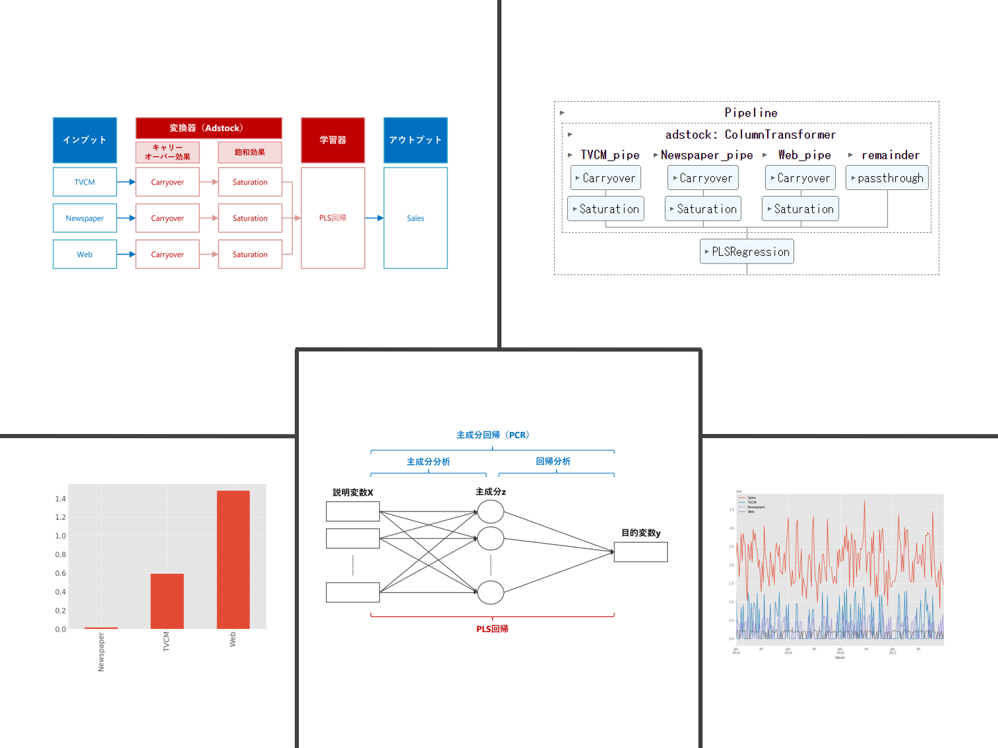
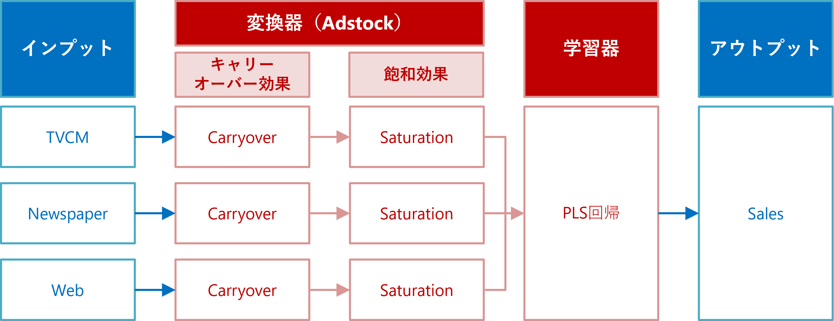
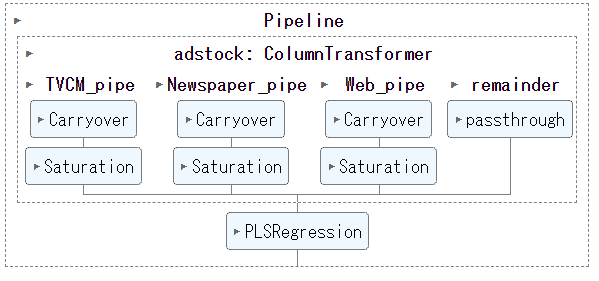
ちなみに、アドストック（Ad Stock）を考慮するとは、飽和効果（収穫逓減）とキャリーオーバー（Carryover）効果を考慮するということです。具体的には、Pythonのscikit-learn（sklearn）のパイプラインを、以下のように構築しました。

利用するデータセット（前回と同じ）

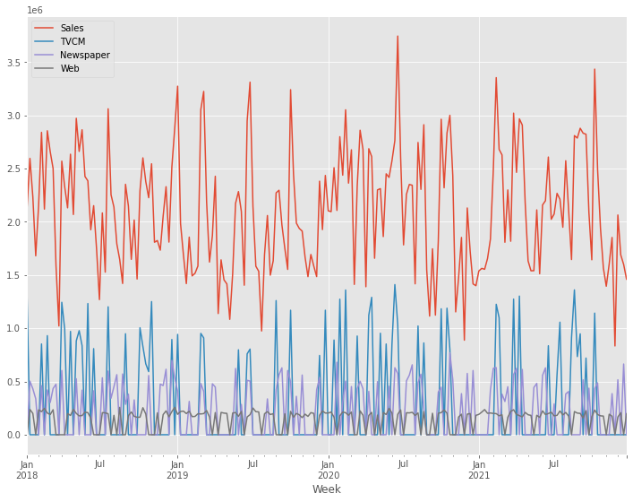
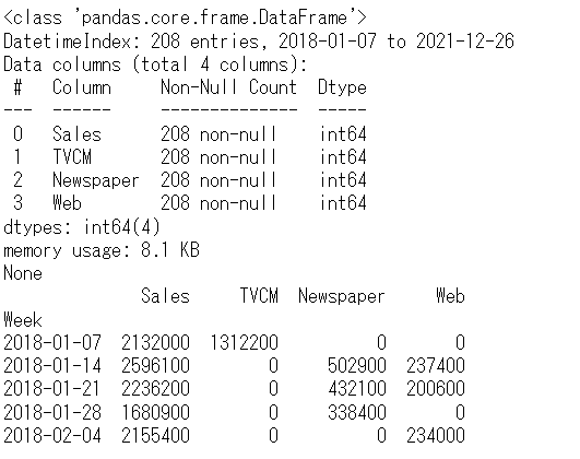
今回利用するデータセットの変数です。

• Week：週
• Sales：売上
• TVCM：TV CMのコスト
• Newspaper：新聞の折り込みチラシのコスト
• Web：Web広告のコスト

以下からダウンロードできます。

MMM.csv
https://www.salesanalytics.co.jp/4zdt

アドストック（Ad Stock）

今回は、以下の関数でアドストック（Ad Stock）を表現しモデル構築したいと思います。

• 定率減少型キャリーオーバー効果モデル　※ピークが広告などの投入時
• 指数型飽和モデル（exp_Saturation）

　定率減少型キャリーオーバー効果モデル

ピークが広告などの投入時で徐々に低減する「定率減少型キャリーオーバー効果モデル」を、数式で表現すると、次のようになります。

ハイパーパラメータは、次の2つです。

• L(length)：効果の続く期間　※当期含む
• R(rate)：減衰率

グラフで表現すると、次のようになります。横軸は、広告などを投入した後の経過時間（当期、1期後、2期後、・・・）を表し、縦軸は、効果の大きさを表します。

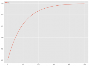
　指数型飽和モデル

「指数型飽和モデル」を数式で表現すると、次のようになります。

$x_ t^{**}=1-e^{-ax_ t^*}$ $x_ t^*$はt期とそれ以前までの広告などの効果の累積（残存効果を足したもの）で、$x_ t^{**}$は指数型飽和モデルで変換した後のt期の値です。

グラフで表現すると、次のようになります。横軸は$x_ t^*$で、縦軸は$x_ t^{**}$です。

この2つの関数に関しては、次の記事でもうちょっと詳しく説明しているので、気になる方は参考にしてください。

ライブラリーやデータセットなどの読み込み

先ずは、必要なライブラリーとデータセットを読み込みます。前回までと同じです。

　必要なライブラリーの読み込み

必要なライブラリーを読み込みます。

以下、コードです。

import numpy as np
import pandas as pd

from scipy.signal import convolve2d

from sklearn.base import BaseEstimator, TransformerMixin
from sklearn.compose import ColumnTransformer
from sklearn.pipeline import Pipeline
from sklearn.model_selection import cross_val_score, TimeSeriesSplit
from sklearn import set_config

from sklearn.cross_decomposition import PLSRegression

from optuna.integration import OptunaSearchCV
from optuna.distributions import UniformDistribution, IntUniformDistribution

import matplotlib.pyplot as plt
plt.style.use('ggplot') #グラフスタイル
plt.rcParams['figure.figsize'] = [12, 9] # グラフサイズ

　データセット（前回と同じ）の読み込み

前回と同じデータセットを読み込みます。

以下、コードです。

# データセット読み込み
url = 'https://www.salesanalytics.co.jp/4zdt'
df = pd.read_csv(url,
                 parse_dates=['Week'],
                 index_col='Week'
                )

# データ確認
print(df.info()) #変数の情報
print(df.head()) #データの一部

# 説明変数Xと目的変数yに分解
X = df.drop(columns=['Sales'])
y = df['Sales']

以下、実行結果です。

ハイパーパラメータ探索

PLS回帰の最適な主成分の数と、キャリーオーバー効果や飽和効果のハイパーパラメータを探索します。

先ずは、Pipeline用変換器を定義します。

以下、コードです。

#
# Pipeline用変換器
#

# 飽和モデル

## 関数の定義
def saturation_func(X: np.ndarray,a):
    return 1 - np.exp(-a*X)

## 変換器の定義
class Saturation(BaseEstimator, TransformerMixin):
    
    # 初期化
    def __init__(self, a=1.0):
        self.a = a #ハイパーパラメータ
    
    # 学習
    def fit(self, X, y=None):
        return self
    
    # 処理（入力→出力）
    def transform(self, X):
        return saturation_func(X,self.a)

# キャリーオーバー効果モデル

## 関数の定義
def carryover_func(X: np.ndarray, rate, length):
    filter = (
        rate ** np.arange(length)
    ).reshape(-1, 1) 
    convolution = convolve2d(X, filter)
    if length > 1 : convolution = convolution[: -(length-1)]
    return convolution

## 変換器の定義
class Carryover(BaseEstimator, TransformerMixin):
    # 初期化
    def __init__(self, rate=0.5, length=1):
        self.rate = rate #ハイパーパラメータ
        self.length = length #ハイパーパラメータ
        
    # 学習        
    def fit(self, X, y=None):
        return self
    
    # 処理（入力→出力）
    def transform(self, X: np.ndarray):
        return carryover_func(X, self.rate, self.length)

次に、Pipelineを構築します。

以下、コードです。

#
# Pipeline構築
#

# 変換器（adstock）
adstock = ColumnTransformer(
    [
     ('TVCM_pipe', Pipeline([
                           ('carryover', Carryover()),
                           ('saturation', Saturation())
     ]), ['TVCM']),
     ('Newspaper_pipe', Pipeline([
                           ('carryover', Carryover()),
                           ('saturation', Saturation())
     ]), ['Newspaper']),
     ('Web_pipe', Pipeline([
                           ('carryover', Carryover()),
                           ('saturation', Saturation())
     ]), ['Web']),
    ],
    remainder='passthrough'
)

## 変換器（adstock）→学習器（regression）
MMM_pipe = Pipeline([
    ('adstock', adstock),
    ('regression', PLSRegression())
])

## パイプラインの確認
set_config(display='diagram')   
MMM_pipe

以下、実行結果です。

そして、Pipelineのハイパーパラメータを探索します。

以下、コードです。

#
# ハイパーパラメータ探索
#

# 探索するハイパーパラメータ範囲の設定
params = {
 ## PLS
 'regression__n_components':
    IntUniformDistribution(1, 3),
 ## TVCM
 'adstock__TVCM_pipe__carryover__rate':
    UniformDistribution(0, 1),
 'adstock__TVCM_pipe__carryover__length':
    IntUniformDistribution(1, 6),
 'adstock__TVCM_pipe__saturation__a':
    UniformDistribution(0, 0.01),
 ## Newspaper
 'adstock__Newspaper_pipe__carryover__rate':
    UniformDistribution(0, 1),
 'adstock__Newspaper_pipe__carryover__length':
    IntUniformDistribution(1, 6),
 'adstock__Newspaper_pipe__saturation__a':
    UniformDistribution(0, 0.01),
 ## Web
 'adstock__Web_pipe__carryover__rate':
    UniformDistribution(0, 1),
 'adstock__Web_pipe__carryover__length':
    IntUniformDistribution(1, 6),
 'adstock__Web_pipe__saturation__a':
    UniformDistribution(0, 0.01),
}

# ハイパーパラメータ探索の設定
optuna_search = OptunaSearchCV(
    estimator=MMM_pipe,
    param_distributions=params,
    n_trials=2000,
    cv=TimeSeriesSplit(),
    random_state=0,
    n_jobs=-1
)

# 探索実施
optuna_search.fit(X, y)

# 探索結果
optuna_search.best_params_

以下、実行結果です。

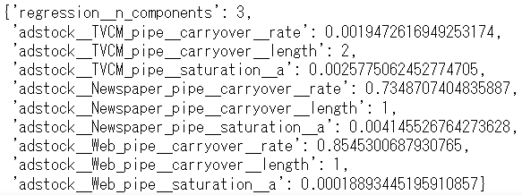
この値をハイパーパラメータに設定し、MMMを全データで構築します。

モデルの構築と予測

　最適ハイパーパラメータで学習

以下、コードです。

#
# 最適ハイパーパラメータで学習
#

# パイプラインのインスタンス
MMM_pipe_best = MMM_pipe.set_params(**optuna_search.best_params_)

# 全データで学習
MMM_pipe_best.fit(X, y)

# R2（決定係数）
MMM_pipe_best.score(X, y)

以下、実行結果です。R2（決定係数）の値です。

　予測の実施

以下、コードです。

#
# 予測の実施
# 

# 目的変数y（売上）の予測
pred = pd.DataFrame(MMM_pipe_best.predict(X),
                    index=X.index,
                    columns=['y'])

# 各媒体による売上の予測

## 値がすべて0の説明変数
X_ = X.copy()
X_.iloc[:,:]=0

## Base
pred['Base'] = MMM_pipe_best.predict(X_)

## 媒体
for i in range(len(X.columns)):
    X_.iloc[:,:]=0
    X_.iloc[:,i]=X.iloc[:,i]
    pred[X.columns[i]] = MMM_pipe_best.predict(X_) - pred['Base']
    
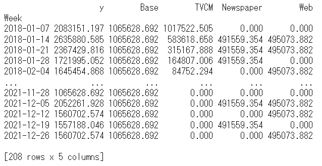
print(pred) #確認

以下、実行結果です。y = Base + TVCM + Newspaper + Webです。

貢献度とマーケティングROIの算定

　貢献度の算定

以下、コードです。

#
# 貢献度の算定
#

# 予測値の補正
correction_factor = y.div(pred['y'], axis=0)   #補正係数
pred_adj = pred.mul(correction_factor, axis=0) #補正後の予測値

# 各媒体の貢献度だけ抽出
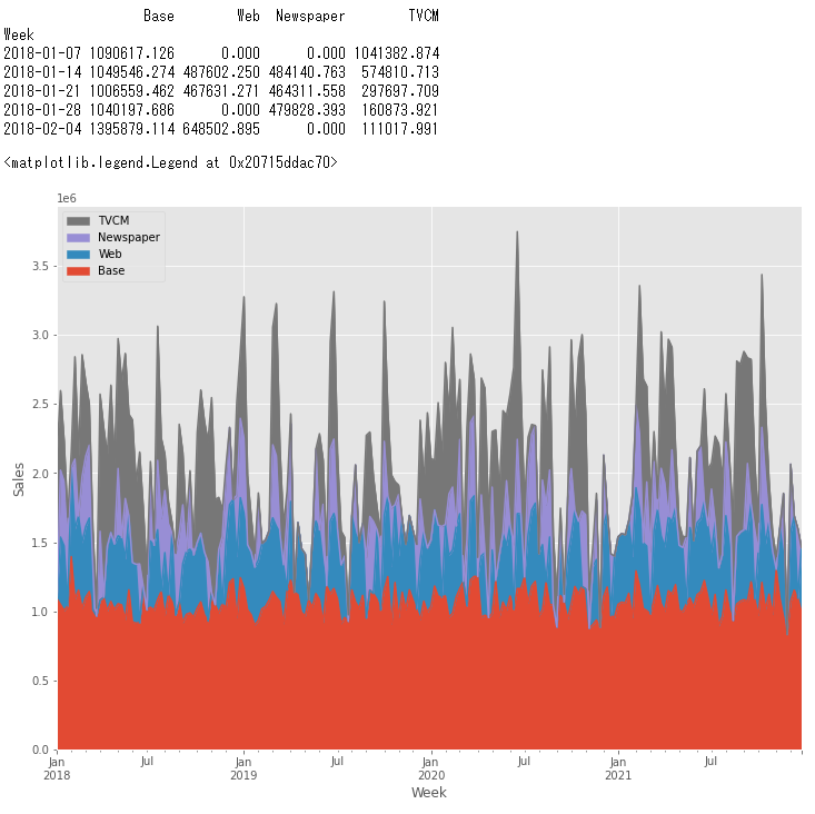
contribution = pred_adj[['Base', 'Web', 'Newspaper', 'TVCM']]

print(contribution.head()) #確認

# グラフ化
ax = (contribution
      .plot.area(
          ylabel='Sales',
          xlabel='Week')
     )
handles, labels = ax.get_legend_handles_labels()
ax.legend(handles[::-1], labels[::-1])

以下、実行結果です。

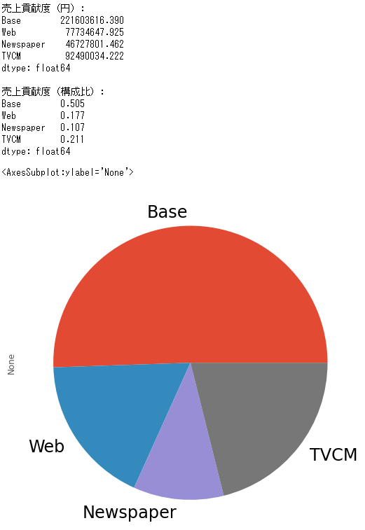
貢献度の構成比の算出します。

以下、コードです。

#
# 貢献度の構成比の算出
#

# 媒体別の貢献度の合計
contribution_sum = contribution.sum(axis=0)

# 集計結果の出力
print('売上貢献度（円）:\n', 
      contribution_sum, 
      sep=''
     )
print()
print('売上貢献度（構成比）:\n', 
      contribution_sum/contribution_sum.sum(), 
      sep=''
     )

# グラフ化
contribution_sum.plot.pie(fontsize=24)

以下、実行結果です。

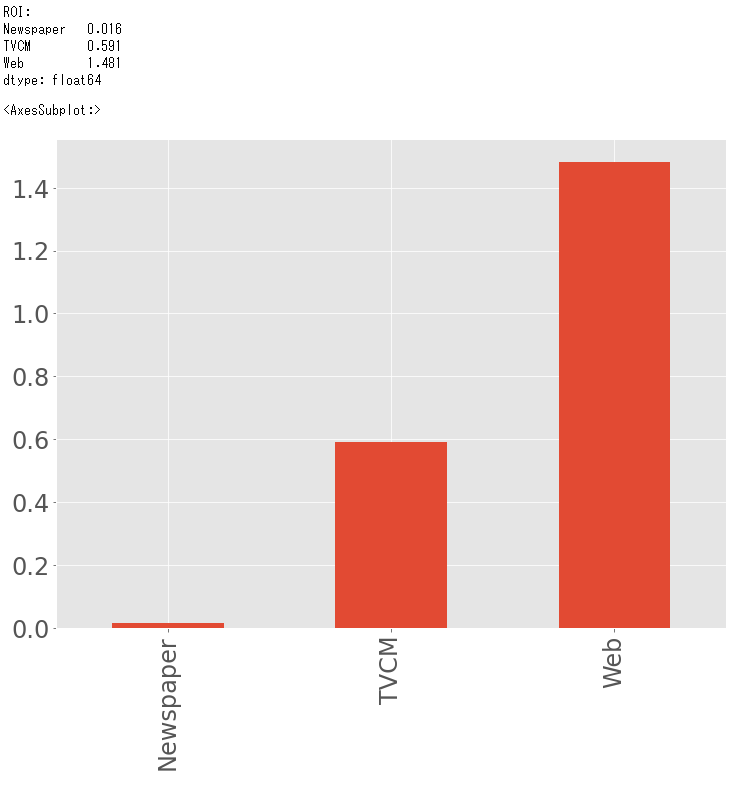
マーケティングROIの算定

以下、コードです。

#
# マーケティングROIの算定
#

# 各媒体のコストの合計
cost_sum = X.sum(axis=0)

# 各媒体のROIの計算
ROI = (contribution_sum.drop('Base', axis=0) - cost_sum)/cost_sum

print('ROI:\n', ROI, sep='') #確認

# グラフ化
ROI.plot.bar(fontsize=24)

以下、実行結果です。

まとめ

今回は、シンプルなAdStockを考慮したPLS回帰によるモデル構築についてお話ししました。

• AdStock非考慮
  
• シンプルなAdStock考慮　→　今回
  
• 色々なAdStock考慮　→　次回

次回は、色々なAdStockを考慮したPLS回帰によるモデル構築についてお話しします。

Pythonによるマーケティングミックスモデリング（MMM：Marketing Mix Modeling）超入門 その13PLS回帰モデルでMMM③（色々なAdStock考慮）