

時系列予測モデルの、予測精度を向上させるために、外生変数(説明変数・特徴量)を利用することがあります。
例えば、需要予測のための価格や将来のプロモーション変数、電力負荷予測のための天気データなどです。
時系列データには、3種類の外生変数(説明変数・特徴量)があります。
- 静的外生変数
- 履歴外生変数
- 未来外生変数
今回は、これらの外生変数をNeuralForecastモデルに組み込み予測する方法について説明します。
NeuralForecastをまだインストールされていない方は、前回の記事で説明していますので、参考にしてください。
Contents [hide]
時系列データの3つの外生変数(exogenous variables)
外生変数とは
外生変数とは、時系列予測モデルなどの統計的モデルにおいて、モデルの外部で値が決まる変数のことです。
外生変数は、モデルに影響を与えるが、モデルから影響を受けない変数と言えます。外生変数は、説明変数や独立変数、特徴量とも呼ばれます。
外生変数の例としては、気温や降水量、景気や消費者信頼感、祝日やイベントなどが挙げられます。
これらの変数は、時系列データに影響を与えるが、時系列データ自体に含まれない変数です。
内生変数とは
外生変数と対照的なものが、内生変数です。内生変数とは、モデルの内部で値が決まる変数のことです。
内生変数は、モデルに影響を与えるとともに、モデルから影響を受ける変数と言えます。内生変数は、従属変数などとも呼ばれます。また、予測対象である目的変数も内生変数です。
内生変数の例としては、消費支出や国民所得、株価や為替レートなどが挙げられます。
これらの変数は、他の変数との関係によって値が決まります。
時系列データの外生変数の種類
時系列データの外生変数の一般的な分類として、以下の3つがあります。
静的外生変数(Static exogenous variables)
時系列データの全期間にわたって一定の値を持つ外生変数です。店舗別や製品別の売上などの複数の時系列データを予測するときに使います。例えば、エリアや製品カテゴリーなどが静的外生変数となります。多くの場合、個々の時系列データ共通の属性データになります。
履歴外生変数(Historic exogenous variables)
時系列データの過去の値やその統計量を外生変数として用いるもので、グレンジャー因果性と関わりの深い変数です。予測対象期間より前の時系列データです。予測対象である目的変数や説明変数の過去のデータや、移動平均などの過去データを計算したものです。
未来外生変数(Future exogenous variables)
時系列データの未来の値やその予測値を外生変数として用いるものです。ざっくり言うと、テーブルデータの説明変数と思っていただければと思います。予測対象期間(要は未来)のデータです。例えば、売上を予測するとき、そのときの売上がそのときのマーケティング変数(キャンペーンなど)や天候などに影響を受けるなら、これらは未来外生変数となります。
これらの3つの外生変数は、明確に意識し分ける必要があります。
NeuralForecastで時系列回帰モデル構築例
利用するデータセット
ある小売チェーンです。在庫管理を改善するため、個店別に需要予測を実施することになりました。
今回、5店舗の売上などの時系列データ(sales_data.csv)と店舗特性データ(static_data.csv)を使い、学習データでモデル構築し、テストデータ(直近7日間)で検証します。
以下からダウンロードできます。
時系列データ(sales_data.csv)と店舗特性データ(static_data.csv)
https://www.salesanalytics.co.jp/u133
売上などの時系列データ(sales_data.csv)
- unique_id:店舗を識別する変数(店舗名)
- ds:日付
- y:売上
- promo:プロモーション実施の有無(1:実施, 0:未実施)
- holiday:休日かどうか(1:休日, 0:平日)
yの売上が、予測対象である目的変数です。
未来外生変数(Future exogenous variables)は、マーケティング変数であるpromoと、カレンダー変数であるholidayです。
マーケティング変数であるpromoは、過去実施分も売上へ影響するため、履歴外生変数(Historic exogenous variables)でもあります。
店舗特性データ(static_data.csv)
- unique_id:店舗を識別する変数(店舗名)
- Type_1:駅前(1:yes, 0:no)
- Type_2:住宅街(1:yes, 0:no)
- Type_3:ロードサイド(1:yes, 0:no)
このデータは、静的外生変数(Static exogenous variables)です。
準備
まず、モジュールを読み込みます。
以下、コードです。
import numpy as np
import pandas as pd

from neuralforecast import NeuralForecast
from neuralforecast.models import (
    RNN,
    LSTM,
    GRU,
    NBEATS,
    NHITS,
)
from neuralforecast.utils import AirPassengersDF

from sklearn.metrics import (
    mean_absolute_error,
    mean_absolute_percentage_error,
    r2_score
)

import matplotlib.pyplot as plt
plt.style.use('ggplot') # グラフのスタイル
次に、データセットを読み込みます。
以下、売上などの時系列データ(sales_data.csv)を読み込むコードです。
# 売上などの時系列データ(sales_data.csv)
df = pd.read_csv('sales_data.csv')
df['ds'] = pd.to_datetime(df['ds'])
print(df)
以下、実行結果です。
    unique_id         ds     y  promo  holiday
0     Store_A 2023-01-08  1383      1        0
1     Store_A 2023-01-09  2204      0        1
2     Store_A 2023-01-10  2193      0        1
3     Store_A 2023-01-11  1512      0        0
4     Store_A 2023-01-12  1180      0        0
..        ...        ...   ...    ...      ...
410   Store_E 2023-03-27  1458      0        1
411   Store_E 2023-03-28  1028      0        0
412   Store_E 2023-03-29   985      0        0
413   Store_E 2023-03-30  1143      0        0
414   Store_E 2023-03-31  1787      0        0

[415 rows x 5 columns]
以下、店舗特性データ(static_data.csv)を読み込むコードです。
# 店舗特性データ(static_data.csv)の読み込み
static_df = pd.read_csv('static_data.csv')
print(static_df)
以下、実行結果です。
  unique_id  Type_1  Type_2  Type_3
0   Store_A       1       0       0
1   Store_B       0       1       0
2   Store_C       1       0       0
3   Store_D       0       0       1
4   Store_E       0       1       0
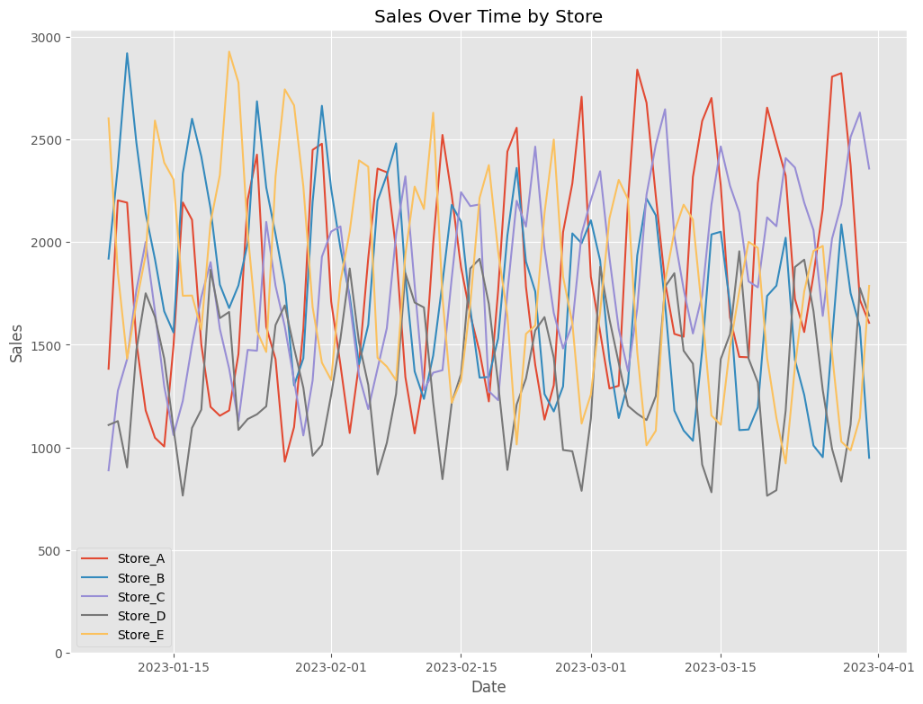
どのようなデータセットなのかグラフで見てみます。
以下、コードです。
# unique_idごとにデータをグループ化
grouped = df.groupby('unique_id')

plt.figure(figsize=(12, 9))

# グループごとにグラフを描画
for name, group in grouped:
    plt.plot(group['ds'], group['y'], label=name)

plt.legend()
plt.title('Sales Over Time by Store')
plt.ylim(bottom=0)
plt.xlabel('Date')
plt.ylabel('Sales')
plt.show()
以下、実行結果です。
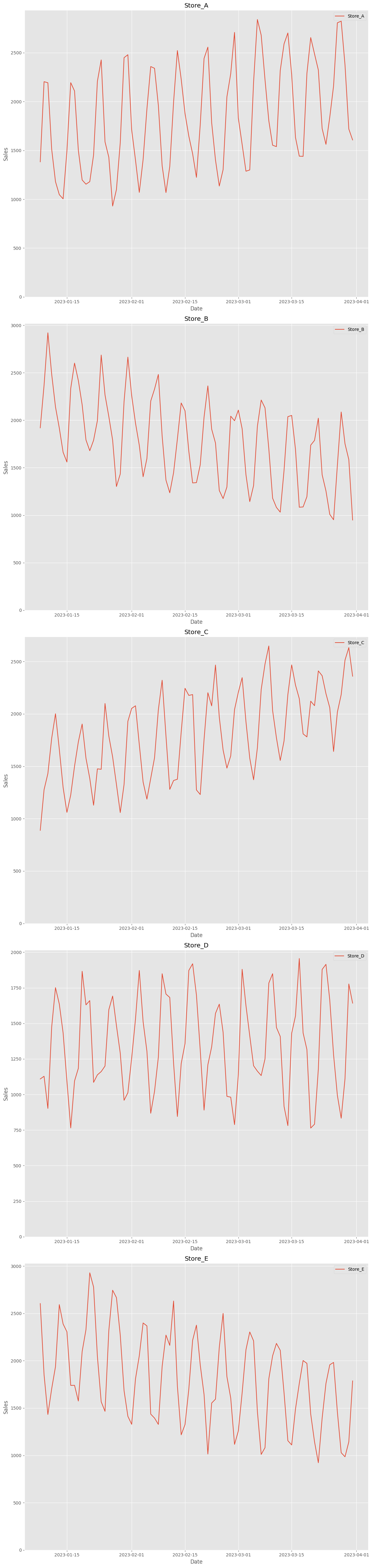
見にくいので、店舗別にプロットします。
以下、コードです。
fig, axes = plt.subplots(nrows=5, figsize=(12, 50))

# グループと軸(作成したサブプロット)を順に反復処理します
for (name, group), ax in zip(grouped, axes):
    ax.plot(group['ds'], group['y'], label=name)
    ax.set_ylim(bottom=0)
    ax.set_title(name)  # タイトルをグループの名前に設定します
    ax.set_xlabel('Date')
    ax.set_ylabel('Sales')
    ax.legend()

plt.tight_layout()
plt.show()
以下、実行結果です。
データセットを、学習用とテスト用に分割します。直近7日間がテストデータです。
以下、コードです。
# 学習データとテストデータに分割
train_df = df[df['ds'] < '2023-03-25']
test_df = df[df['ds'] >= '2023-03-25']

# 予測期間
horizon = 7
1つのモデルで構築する(RNN)
学習データでモデル構築
RNNモデルで、店舗別に売上を予測するモデルを構築します。
以下、コードです。
# モデルのパラメータ
rnn_params = {
    'input_size': 4 * horizon,
    'h': horizon,
    'futr_exog_list':['holiday','promo'],
    'hist_exog_list':['promo'],
    'stat_exog_list':['Type_1', 'Type_2', 'Type_3'],
    'scaler_type':'robust',
    'max_steps': 50,
}

# モデルのインスタンス
rnn_model = RNN(**rnn_params)
nf = NeuralForecast(models=[rnn_model], freq='D')

# モデルの学習
nf.fit(df=train_df, static_df=static_df)
テストデータで検証
テストデータの予測を行い、精度評価指標としてMAPE、MAE、R2を出力します。
以下、コードです。
# 計算結果を格納
results = []

# 'unique_id'ごとに計算
for unique_id in test_df['unique_id'].unique():
    y_true = test_df[test_df['unique_id'] == unique_id]['y']
    y_pred = Y_hat_df[Y_hat_df.index == unique_id]['RNN']

    mae = mean_absolute_error(y_true, y_pred)
    mape = mean_absolute_percentage_error(y_true, y_pred)
    r2 = r2_score(y_true, y_pred)

    results.append([unique_id, mae, mape, r2])

results_df = pd.DataFrame(
    results,
    columns=['unique_id', 'MAE', 'MAPE', 'R2'])

print(results_df)
以下、実行結果です。
  unique_id         MAE      MAPE        R2
0   Store_A  329.890224  0.153269  0.348956
1   Store_B  279.431710  0.236446  0.433639
2   Store_C  306.979510  0.143645 -0.245875
3   Store_D   97.573975  0.076813  0.899395
4   Store_E  219.920253  0.167454  0.631261
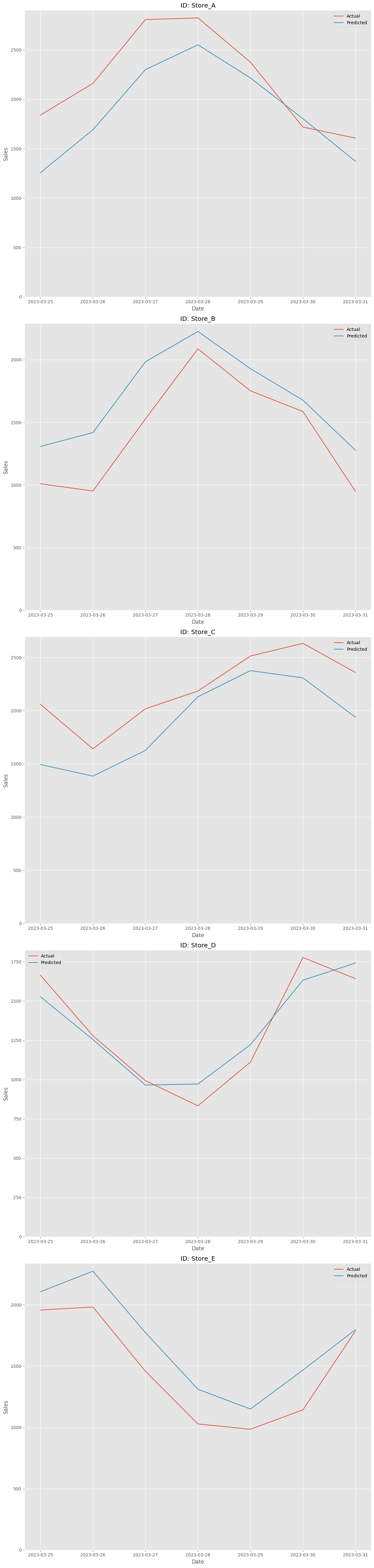
予測値と実測値をプロットします。
以下、コードです。
# 各unique_idごとにサブプロットを生成
fig, axes = plt.subplots(nrows=len(Y_hat_df.index.unique()), figsize=(12, 50))

for ax, unique_id in zip(axes, Y_hat_df.index.unique()):
  # 現在のunique_idのデータを選択
  actual = test_df[test_df["unique_id"] == unique_id]
  predicted = Y_hat_df.loc[unique_id]

  # 実際のデータと予測データを同じプロットに描画
  ax.plot(actual["ds"], actual["y"], label='Actual')
  ax.plot(predicted["ds"], predicted["RNN"], label='Predicted')

  # タイトルとラベルの設定
  ax.set_title(f"ID: {unique_id}")
  ax.set_xlabel('Date')
  ax.set_ylabel('Sales')
  ax.set_ylim(bottom=0)
  ax.legend()

plt.tight_layout()
plt.show()
以下、実行結果です。
複数のモデルで構築する
先ほどはRNNモデルで予測モデルを構築してみました。
ここでは、以下の複数の時系列深層学習アルゴリズム(モデルタイプ)で予測モデルを構築していきます。
| モデルタイプ | 説明 |
|---|---|
| RNN | RNNは、時系列データやシーケンスデータを扱うのに適したニューラルネットワークです。連続するデータ間の時間的な依存関係をモデル化することができます。 |
| LSTM | LSTMはRNNの一種で、長期的な依存関係をより効果的に学習できるように設計されています。これにより、RNNが通常持つ短期的な依存関係の制限を克服します。 |
| GRU | GRUはLSTMに似ていますが、より単純な構造を持っています。これにより、計算効率が向上し、小規模なデータセットでの性能が改善されることがあります。 |
| NBEATS | NBEATSは完全に接続されたフィードフォワードニューラルネットワークです。時系列データの基本的なパターンを捉えるために、基底展開法を用いています。 |
| NHITS | NHITSはNBEATSに触発されたモデルで、階層的なアプローチを取り入れています。これにより、異なる時間スケールでのパターンをより効果的に捉えることができます。 |
学習データでモデル構築
複数の深層学習アルゴリズムで、店舗別に売上を予測するモデルを構築します。
以下、コードです。
# 共通パラメータの定義
common_params = {
    'input_size': 4 * horizon,  # Reduced input_size
    'h': horizon,
    'futr_exog_list':['holiday','promo'],
    'hist_exog_list':['promo'],
    'stat_exog_list':['Type_1', 'Type_2', 'Type_3'],
    'scaler_type':'robust',
    'max_steps': 50,
}

# モデルのインスタンス
model_types = [RNN, LSTM, GRU, NBEATS, NHITS]
models = [model_type(**common_params) for model_type in model_types]
nf = NeuralForecast(models=models, freq='D')

# モデルの学習
nf.fit(df=train_df, static_df=static_df)
テストデータで検証
テストデータの予測を行い、精度評価指標としてMAPE、MAE、R2を出力します。
以下、コードです。
# モデルで予測を行う
Y_hat_dfs = nf.predict(futr_df=test_df)

# 各モデルタイプのエラーメトリクスを計算する
results = []
model_names = [model.__name__ for model in model_types]
for model_name in model_names:
    for unique_id in test_df['unique_id'].unique():
        y_true = test_df[test_df['unique_id'] == unique_id]['y']
        y_pred = Y_hat_dfs.loc[unique_id, model_name]

        mae = mean_absolute_error(y_true, y_pred)
        mape = mean_absolute_percentage_error(y_true, y_pred)
        r2 = r2_score(y_true, y_pred)

        results.append([model_name, unique_id, mae, mape, r2])

# 結果を保存するデータフレームを作成する
results_df = pd.DataFrame(
    results,
    columns=['Model', 'unique_id', 'MAE', 'MAPE', 'R2'])

print(results_df)
以下、実行結果です。
     Model unique_id         MAE      MAPE        R2
0      RNN   Store_A  329.890224  0.153269  0.348956
1      RNN   Store_B  279.431710  0.236446  0.433639
2      RNN   Store_C  306.979510  0.143645 -0.245875
3      RNN   Store_D   97.573975  0.076813  0.899395
4      RNN   Store_E  219.920253  0.167454  0.631261
5     LSTM   Store_A  364.737148  0.179588  0.309094
6     LSTM   Store_B  376.027291  0.321956  0.000937
7     LSTM   Store_C  348.925746  0.163112 -0.730577
8     LSTM   Store_D  138.413775  0.113563  0.810342
9     LSTM   Store_E  313.125610  0.233442  0.367974
10     GRU   Store_A  161.496390  0.076327  0.865642
11     GRU   Store_B  221.074829  0.193989  0.635155
12     GRU   Store_C  152.249023  0.068595  0.662957
13     GRU   Store_D  133.832223  0.112466  0.822676
14     GRU   Store_E  115.422311  0.090725  0.894941
15  NBEATS   Store_A   86.927141  0.041711  0.949431
16  NBEATS   Store_B  125.884992  0.095745  0.883273
17  NBEATS   Store_C  143.528216  0.066312  0.754716
18  NBEATS   Store_D  106.228838  0.091964  0.836377
19  NBEATS   Store_E   70.888096  0.050452  0.959743
20   NHITS   Store_A  104.677124  0.052887  0.922507
21   NHITS   Store_B  193.078369  0.164124  0.706014
22   NHITS   Store_C  119.017003  0.057181  0.826427
23   NHITS   Store_D  111.776986  0.092693  0.839330
24   NHITS   Store_E   53.991411  0.037689  0.959233
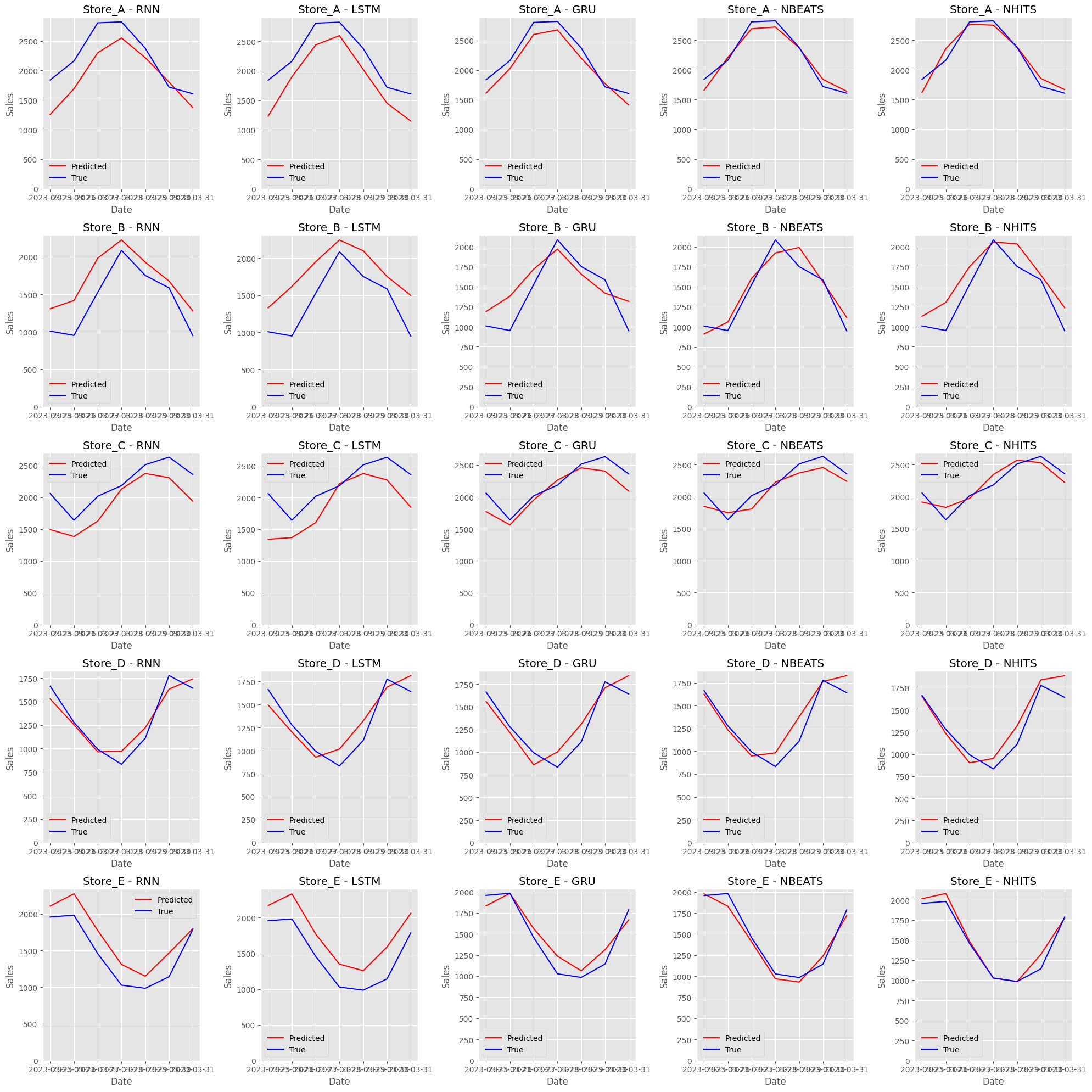
予測値と実測値をプロットします。
以下、コードです。
# 一意の店舗名(識別子)を取得
unique_ids = test_df['unique_id'].unique()

# サブプロットの設定
fig, axes = plt.subplots(
    nrows=len(unique_ids),
    ncols=len(model_names),
    figsize=(20, 20))

# すべてのunique_ids(各異なるストア)でループ
for i, unique_id in enumerate(unique_ids):
    # このストアの真の値を取得
    y_true = test_df[test_df['unique_id'] == unique_id]['y']
    dates = test_df[test_df['unique_id'] == unique_id]['ds']

    # すべてのモデルでループ
    for j, model_name in enumerate(model_names):
        # このストアの予測値を取得してプロット
        y_pred = Y_hat_dfs.loc[unique_id, model_name]
        axes[i, j].plot(dates, y_pred, label='Predicted', color='red')

        # 真の値をプロット
        axes[i, j].plot(dates, y_true, label='True', color='blue')

        # タイトルとラベルの設定
        axes[i, j].set_title(f'{unique_id} - {model_name}')
        axes[i, j].set_xlabel('Date')
        axes[i, j].set_ylabel('Sales')
        axes[i, j].set_ylim(bottom=0)
        axes[i, j].legend()

# レイアウトを調整してプロットを表示
plt.tight_layout()
plt.show()
以下、実行結果です。クリックすると拡大します。
まとめ
今回は、時系列予測モデルの構築において外生変数の重要性とその活用方法について解説しました。
外生変数は、予測モデルの精度を向上させるために不可欠であり、静的外生変数、履歴外生変数、未来外生変数の3種類が存在します。
具体的な例として、小売チェーンの売上データと店舗特性データを用いたモデル構築の過程を紹介し、RNNを含む複数の深層学習モデルを用いた検証方法を示しました。
これらの知識は、ビジネスにおけるデータ駆動型の意思決定をサポートし、より精度の高い予測を可能にするために重要です。