非線形計画問題の大域的最適化は、工学や経済学など様々な分野で重要な役割を果たしています。特に、問題の規模が大きくなると、局所的な最適解ではなく、大域的な最適解を見つけることが求められます。

これまでの連載では、Pythonを使った非線形計画問題の定式化や、SciPyを使った最適化の方法について学びました。しかし、問題の規模が大きくなると、SciPyでは計算時間が長くなったり、メモリ不足になったりすることがあります。

そこで、今回は、大規模な非線形最適化問題に特化したPythonライブラリ、CyIPOPTを紹介します。CyIPOPTは、Interior Point OPTimizer (IPOPT) をPythonから利用するためのインターフェースで、高速かつメモリ効率の良い最適化が可能です。

CyIPOPTとは？

CyIPOPTは、Cythonを使って記述されたPythonモジュールで、IPOPTの機能をPythonから利用できるようにしたものです。IPOPTは、内点法と呼ばれる手法を用いて、大規模な非線形最適化問題を高速に解くことができます。

IPOPTは、C++で記述されたソフトウェアで、そのままではPythonから利用することができません。CyIPOPTは、IPOPTとPythonの間に位置し、IPOPTの機能をPythonから利用できるようにするためのインターフェースの役割を果たしています。

CyIPOPTには、以下のような特徴があります。

大規模な非線形最適化問題に適している
CyIPOPTは、IPOPTの機能を利用しているため、変数の数が数千から数万にもおよぶ大規模な問題を解くことができます。

スパース行列の取り扱いが可能
非線形最適化問題では、ヤコビ行列やヘッセ行列がスパース（疎行列）になることが多くあります。CyIPOPTは、スパース行列を効率的に取り扱うことができるため、メモリ使用量を削減できます。

制約付き最適化と制約なし最適化の両方に対応
CyIPOPTは、等式制約や不等式制約を含む制約付き最適化問題と、制約条件のない最適化問題の両方を解くことができます。

SciPyの最適化モジュール（scipy.optimize）も、非線形最適化問題を解くことができますが、CyIPOPTとは以下のような違いがあります。

問題の規模
SciPyは、中小規模の問題に適しているのに対し、CyIPOPTは大規模な問題に適しています。

スパース行列の取り扱い
SciPyは、スパース行列を直接取り扱うことができませんが、CyIPOPTはスパース行列を効率的に取り扱うことができます。

計算速度とメモリ効率
大規模な問題では、CyIPOPTの方がSciPyよりも計算速度が速く、メモリ効率が良いです。

このように、CyIPOPTは、大規模な非線形最適化問題を解くのに適したライブラリです。

特に、問題の規模が大きい場合や、スパース行列を含む問題を解く場合には、CyIPOPTを使うことで、効率的に最適解を求めることができます。

CyIPOPTの使い方

ここでは、CyIPOPTのインストール方法と基本的な使い方について説明します。

　CyIPOPTのインストール

condaでインストールするときは、以下です。

conda install -c conda-forge cyipopt

インストールが上手くいかない場合、pipでインストールしたいもしくはIpoptそのものをインストールしたい場合、以下を参考にしていただければと思います。OSなどによりやり方が変わります。

cyipopt Installation
https://cyipopt.readthedocs.io/en/stable/install.html

　CyIPOPTの基本的な使い方

CyIPOPTを使って最適化問題を解くには、以下の手順を実行します。

• Step.1 目的関数の定義 ：最小化したい目的関数を定義します。目的関数は、Pythonの関数として定義します。
• Step.2 制約条件の定義 ：最適化問題に制約条件がある場合は、制約条件を定義します。制約条件も、Pythonの関数として定義します。
• Step.3 オプションの設定 ：最適化アルゴリズムのオプション（収束判定条件、最大反復回数など）を設定します。
• Step.4 最適化の実行 ：minimize_ipopt関数を呼び出して、最適化を実行します。

以下の最適化問題を例に簡単に説明していきます。

　　Step.1　目的関数の定義

CyIPOPTを使って最適化問題を解くには、まず目的関数を定義する必要があります。

目的関数は、最小化（または最大化）したい関数で、Pythonの関数として定義します。

例えば、以下のように2次関数を目的関数として定義できます。

def objective(x):
    return (x[0] - 1)**2 + (x[1] - 2.5)**2

SciPy（scipy.optimize）と同じ方法で定義されます。

目的関数の勾配（gradient）を指定することで、最適化アルゴリズムの収束速度を向上させることができます。

勾配（gradient）は、目的関数の各変数での偏微分値をNumPyの配列として返す関数で指定します。

以下、先ほどの目的関数の勾配（gradient）です。

def gradient(x):
    return np.array([2*(x[0] - 1), 2*(x[1] - 2.5)])

こちらも、SciPy（scipy.optimize）と同じ方法で定義されます。

また、定義するかどうかはオプションです。定義しなくても問題ございません。

　　Step.2　制約条件の定義

最適化問題に制約条件がある場合は、制約条件を定義する必要があります。なければ、定義する必要がございません。

制約条件は、等式制約と不等式制約の2種類があります。

制約条件は、制約式の左辺をPythonの関数として定義します。

def constraint1(x):
    return 5 - x[0]**2 - x[1]**2  # 不等式制約

def constraint2(x):
    return x[0]**2 - x[1] - 1  # 不等式制約

SciPy（scipy.optimize）と同じ方法で定義されます。

最適化アルゴリズムの収束速度を向上させたいのであれば、必須ではないですが、制約条件のヤコビアンを指定するといいでしょう。

ヤコビアンは、制約条件の各変数での偏微分値をNumPyの配列として返す関数で指定します。

def constraint1_jac(x):
    return np.array([-2*x[0], -2*x[1]])

def constraint2_jac(x):
    return np.array([2*x[0], -1])

こちらも、SciPy（scipy.optimize）と同じ方法で定義されます。

また、定義するかどうかはオプションです。制約条件のみの定義でも問題ございません。

変数の取り得る値の範囲を指定することができます。

変数の範囲は、各変数の下限と上限をタプルのリストとして指定します。

bounds = [(0, None), (0, None)]  # すべての変数が0以上

こちらも、SciPy（scipy.optimize）と同じ方法で定義されます。

また、定義するかどうかはオプションですが、皆目見当が付かないとき以外は、何かしら設定した方がいいでしょう。

　　Step.3　オプションの設定

 最適化アルゴリズムの動作を制御するためのオプションを指定することができます。

オプションは、辞書形式で指定します。

options = {
    'disp': 3,  # 表示レベル
}

このオプションは、CyIPOPT独自のオプションのため、SciPy（scipy.optimize）とは異なります。

　　Step.4　最適化の実行

初期値を設定します。

初期値は、最適化アルゴリズムの開始点となる変数の値で、NumPyの配列として指定します。

例えば、以下のように初期値を設定できます。

x0 = np.array([1.0, 1.0])

SciPy（scipy.optimize）と同じ方法で定義されます。

最後に、minimize関数を呼び出すことで、制約条件付き最適化問題や、勾配情報を利用した最適化問題を解くことができます。

result = minimize(
    objective, 
    x0, 
    jac=gradient, 
    bounds=bounds, 
    constraints=cons, 
    options=options)

SciPy（scipy.optimize）と似ていますが、やや異なります。

　CyIPOPTの入力と出力

最適化の実行をする前に、必ず定義しなければならないものと、そうでないもの（任意で定義）するもので分かれます。

必ず定義するもの

• 目的関数の定義（SciPy（scipy.optimize）と同じ）
• 初期値の設定（SciPy（scipy.optimize）と同じ）

任意で定義するもの（オプション）

• 目的関数の勾配（SciPy（scipy.optimize）と同じ）
• 制約条件の定義（SciPy（scipy.optimize）と同じ）
• 制約条件のヤコビアン（SciPy（scipy.optimize）と同じ）
• 変数の範囲（上下限）の設定（SciPy（scipy.optimize）と同じ）
• 最適化オプションの設定

目的関数や制約条件の定義する方法がSciPy（scipy.optimize）と共通しているのが特徴です。

そのため、SciPy（scipy.optimize）で問題を定義した最適化問題を、CyIPOPTで解くことは非常に簡単です。

CyIPOPTの出力は、OptimizeResultオブジェクトとして返されます。このオブジェクトには、以下の属性が含まれています。

• x：最適解
• fun：最適解での目的関数の値
• status：最適化の終了状態（成功なら0）
• message：最適化の終了メッセージ
• nfev：目的関数の評価回数
• njev：ヤコビ行列の評価回数
• nit：反復回数

　CyIPOPTのオプション

CyIPOPTの出力は、OptimizeResultオブジェクトとして返され、以下の属性が含まれています。

• x: 最適解の変数値
• fun: 最適解での目的関数の値
• success: 最適化が成功したかどうかを示すブール値
• status: 最適化の終了状態を示す整数値
• message: 最適化の終了メッセージ
• nfev: 目的関数の評価回数
• njev: ヤコビアンの評価回数
• nit: 反復回数

以下、コード例です。

print("最適解:", result.x)
print("目的関数の最小値:", result.fun)
print("最適化の成否:", result.success)
print("終了状態:", result.status)
print("終了メッセージ:", result.message)
print("目的関数の評価回数:", result.nfev)
print("ヤコビアンの評価回数:", result.njev)
print("反復回数:", result.nit)

オプションの設定には注意が必要です。不適切なオプションを設定すると、最適化アルゴリズムが収束しなかったり、数値的に不安定になったりする可能性があります。

オプションの設定には、最適化アルゴリズムに関する知識と経験が必要です。

　簡単な実行例

今説明していた、以下の非線形計画問題を解いてみます。

以下、コードです。

from cyipopt import minimize_ipopt as minimize
import numpy as np

# 目的関数の定義
def objective(x):
    return (x[0] - 1)**2 + (x[1] - 2.5)**2

# 目的関数の勾配
def gradient(x):
    return np.array([2*(x[0] - 1), 2*(x[1] - 2.5)])

# 制約条件1の定義
def constraint1(x):
    return 5 - x[0]**2 - x[1]**2

# 制約条件1のヤコビアン
def constraint1_jac(x):
    return np.array([-2*x[0], -2*x[1]])

# 制約条件2の定義
def constraint2(x):
    return x[0]**2 - x[1] - 1

# 制約条件2のヤコビアン
def constraint2_jac(x):
    return np.array([2*x[0], -1])

# 制約条件の設定
cons = [{'type': 'ineq',
         'fun': constraint1,
         'jac': constraint1_jac},
        {'type': 'ineq',
         'fun': constraint2,
         'jac': constraint2_jac}]

# 初期値
x0 = np.array([1.0, 1.0])

# 変数の範囲: すべての変数が0以上
bounds = [(0, None), (0, None)]

# 最適化オプション
options = {
    'disp': 3,  # 表示レベル
}

# 最適化問題を解く
result = minimize(
    objective, 
    x0, 
    jac=gradient, 
    bounds=bounds, 
    constraints=cons, 
    options=options)

print("最適解:", result.x)
print("目的関数の最小値:", result.fun)

以下、実行結果です。

最適解: [1.60048518 1.56155282]
目的関数の最小値: 1.2412655640868377

同じことを、SciPy（scipy.optimize）で実施してみます。コードはほぼ一緒で、最後の方にある最適化オプションと最適化問題を解くあたりのみ異なります。

以下、コードです。

from scipy.optimize import minimize
import numpy as np

# 目的関数の定義
def objective(x):
    return (x[0] - 1)**2 + (x[1] - 2.5)**2

# 目的関数の勾配
def gradient(x):
    return np.array([2*(x[0] - 1), 2*(x[1] - 2.5)])

# 制約条件1の定義
def constraint1(x):
    return 5 - x[0]**2 - x[1]**2

# 制約条件1のヤコビアン
def constraint1_jac(x):
    return np.array([-2*x[0], -2*x[1]])

# 制約条件2の定義
def constraint2(x):
    return x[0]**2 - x[1] - 1

# 制約条件2のヤコビアン
def constraint2_jac(x):
    return np.array([2*x[0], -1])

# 制約条件の設定
cons = [{'type': 'ineq',
         'fun': constraint1,
         'jac': constraint1_jac},
        {'type': 'ineq',
         'fun': constraint2,
         'jac': constraint2_jac}]

# 初期値
x0 = np.array([1.0, 1.0])

# 変数の範囲: すべての変数が0以上
bounds = [(0, None), (0, None)]

# 最適化オプション
options = {
    'disp': False,  # 表示レベル
}

# 最適化問題を解く
result = minimize(
    objective, 
    x0, 
    jac=gradient, 
    bounds=bounds, 
    constraints=cons, 
    options=options, 
    method='SLSQP')

print("最適解:", result.x)
print("目的関数の最小値:", result.fun)

以下、実行結果です。

最適解: [1.60048518 1.56155282]
目的関数の最小値: 1.2412655640868377

CyIPOPTで非線形計画問題を解く

CyIPOPTを使って、ちょっと複雑な非線形計画問題を解いていきます。第1回でSciPy（scipy.optimize）で解いた問題です。

　　制約なし非線形計画問題

第1回から扱っている、多数の局所最適解を持つことが知られている以下のAckley関数を目的関数にし最小化する例を示します。最適解は $(x_0,x_1)=(-3,4)$ で、最適値は 0 です。

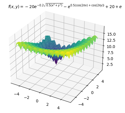
以下、コードです。変数の上下限制約のみ入れています。

from cyipopt import minimize_ipopt as minimize
import numpy as np

# 目的関数の定義
def objective(x):
    a = 20
    b = 0.2
    c = 2 * np.pi
    n = len(x)
    x_offset = np.array([x[0] + 3, x[1] - 4])
    sum_sq_term = -a * np.exp(-b * np.sqrt(sum(x_offset**2) / n))
    cos_term = -np.exp(sum(np.cos(c * x_offset) / n))
    return sum_sq_term + cos_term + a + np.e
        
# 最適化する変数の下限と上限
bounds = ((-5, 5), (-5, 5))

# 初期値
x0 = [0, 0]

# 最適化
res = minimize(
    objective, 
    x0, 
    bounds=bounds)

# 最適解
print("最適解:", res.x) 
print("目的関数の最小値:", res.fun)

以下、実行結果です。

最適解: [-0.01578627  0.02107524]
目的関数の最小値: 10.120350743632672

以下は小数点2桁目を四捨五入した結果です。

• 最適解（Optimal solution）：$(x_0,x_1)=(-0.0,0.0)$
• 最適値（Optimal value）：10.1

　　制約付き非線形計画問題

こちらも第1回から扱っている、、以下の非線形計画問題を扱います。最適解は $(x_0,x_1)=(1,1)$ で、最適値は $0$ です。

以下、コードです。

from cyipopt import minimize_ipopt as minimize
import numpy as np

# 目的関数の定義
def objective(x):
    return (1 - x[0])**2 + 100 * (x[1] - x[0]**2)**2

# 制約条件の定義
def constraint1(x):
    return x[0] - 2 * x[1] - 2

def constraint2(x):
    return np.exp(x[1]) - 8

def constraint3(x):
    return x[0]**2 + x[1]**2 - 10

cons = ({'type': 'ineq', 'fun': constraint1},
        {'type': 'ineq', 'fun': constraint2},
        {'type': 'ineq', 'fun': constraint3})
        
# 最適化する変数の下限と上限
bounds = ((-5, 5), (-5, 5))

# 初期値
x0 = [0, 0]

# 最適化
res = minimize(
    objective, 
    x0, 
    constraints=cons, 
    bounds=bounds)

# 最適解
print("最適解:", res.x) 
print("目的関数の最小値:", res.fun)

以下、実行結果です。

最適解: 5. 2.07944154]
目的関数の最小値: 52551.20230226535

以下は小数点2桁目を四捨五入した結果です。

• 最適解（Optimal solution）：$(x_0,x_1)=(5.0,2.1)$
• 最適値（Optimal value）：52551.2

CyIPOPTを利用した大域的最適化のハイブリッド手法

CyIPOPTは局所的最適化アルゴリズムであるため、非線形計画問題の大域的最適解を保証することはできません。

しかし、CyIPOPTをメタヒューリスティクスや決定論的手法（グローバルサーチ）と組み合わせることで、大域的最適解を効率的に探索することができます。

ここでは、CyIPOPTを利用した大域的最適化のハイブリッド手法について説明します。

第4回でSciPyで実施していたローカルサーチの個所を、CyIPOPTのローカルサーチで置き換えただけです。

今回は、メタヒューリスティクスとローカルサーチを組み合わせで実施する方法について説明します。

アルゴリズムの設計方針

• グローバル探索の実施: メタヒューリスティックスを使用して、探索空間全体から良好な解の候補を見つけ出します。
• ローカルサーチの適用: メタヒューリスティックスで見つけた解を初期点として、ローカルサーチを適用し解の質をさらに向上させます。
• 結果の比較と更新: ローカルサーチ後の解が以前の解よりも良い場合、最良解を更新します。
• 反復処理: 上記のプロセスを繰り返し、改善が見られなくなるまで、または特定の反復回数に達するまで実行します。

先ず、先ほど登場した多数の局所最適解を持つことが知られている以下のAckley関数を目的関数にし最小化する例を示します。最適解は $(x_0,x_1)=(-3,4)$ で、最適値は 0 です。

以下、コードです。変数の上下限制約のみ入れています。

import numpy as np
import pygmo as pg
from cyipopt import minimize_ipopt as minimize

#
# 目的関数などの定義
#

# 目的関数
def objective(x):
    a = 20  # 定数a
    b = 0.2  # 定数b
    c = 2 * np.pi  # 定数c
    n = len(x)  # 入力xの要素数
    x_offset = np.array([x[0] + 3, x[1] - 4])  # xのオフセット調整
    sum_sq_term = -a * np.exp(-b * np.sqrt(sum(x_offset**2) / n))  # 二乗の合計項
    cos_term = -np.exp(sum(np.cos(c * x_offset) / n))  # cos項
    return sum_sq_term + cos_term + a + np.e  # 関数の合計値を返す

# 最適化する変数の下限と上限
bounds = ((-5, 5), (-5, 5))

#
# メタヒューリスティクスの設定
#

# PyGMOで使用するカスタム問題クラス
class CustomProblem:
    def fitness(self, x):
        return [objective(x)]  # 評価関数
    
    def get_bounds(self):
        return ([-100, -100], [100, 100])  # xの上下界を設定

# PyGMO問題オブジェクトを作成
prob = pg.problem(CustomProblem())

# アルゴリズムを設定
algo = pg.algorithm(pg.de(gen=100))

# 初期個体群を生成
pop = pg.population(prob, 20)

#
# 最適解を探索
#

for i in range(10):
    pop = algo.evolve(pop)  # メタヒューリスティック
    best_x = pop.champion_x  # 最良解
    best_f = pop.champion_f[0]  # 最良評価値
    
    # ローカルサーチ
    result = minimize(
        objective, 
        best_x, 
        bounds=bounds,
        constraints=cons)

    # 最適解の更新  
    if result.fun < best_f:  # もし改善されたら、
        best_x = result.x  # 最良解を更新
        best_f = result.fun  # 最良評価値を更新

# 結果を表示
print("最適解:", best_x)
print("目的関数の最小値: ", best_f)

以下、実行結果です。

最適解: [-3.00000002 4.00000001]
目的関数の最小値:  <span>6.271652752687373e-08</span>

以下は小数点2桁目を四捨五入した結果です。

• 最適解（Optimal solution）：$(x_0,x_1)=(-3.0,4.0)$
• 最適値（Optimal value）：0.0

次に、先ほど登場した

以下の非線形計画問題を扱います。最適解は $(x_0,x_1)=(1,1)$ で、最適値は $0$ です。

メタヒューリスティクスでは制約条件はペナルティとして目的関数に組み込み最適化します。

以下、コードです。

import numpy as np
import pygmo as pg
from cyipopt import minimize_ipopt as minimize

#
# 目的関数などの定義
#

# 目的関数
def objective(x):
    return (1 - x[0])**2 + 100 * (x[1] - x[0]**2)**2

# 制約条件の定義
def constraint1(x):
    return x[0] - 2 * x[1] - 2

def constraint2(x):
    return np.exp(x[1]) - 8

def constraint3(x):
    return x[0]**2 + x[1]**2 - 10

cons = ({'type': 'ineq', 'fun': constraint1},
        {'type': 'ineq', 'fun': constraint2},
        {'type': 'ineq', 'fun': constraint3})

# 最適化する変数の下限と上限
bounds = ((-5, 5), (-5, 5))

# 制約違反のペナルティを計算する関数
def calculate_penalty(x):
    c1 = constraint1(x)
    c2 = constraint2(x)
    c3 = constraint3(x)
    penalty = max(0, c1) + max(0, c2) + max(0, c3)
    return penalty

#
# メタヒューリスティクスの設定
#

# PyGMOで使用するカスタム問題クラス
class CustomProblem:
    def fitness(self, x):
        # 目的関数値とペナルティを合計
        obj = objective(x)
        penalty = calculate_penalty(x)
        return [obj + penalty * 1e10]  # ペナルティの重みを調整

    def get_bounds(self):
        return ([-5, -5], [5, 5])

    def get_nobj(self):
        return 1

# PyGMO問題オブジェクトを作成
prob = pg.problem(CustomProblem())

# アルゴリズムを設定
algo = pg.algorithm(pg.de(gen=100))

# 初期個体群を生成
pop = pg.population(prob, 20)

#
# 最適解を探索
#

for i in range(10):
    pop = algo.evolve(pop)  # メタヒューリスティック
    best_x = pop.champion_x  # 最良解
    best_f = pop.champion_f[0]  # 最良評価値
    
    # ローカルサーチ
    result = minimize(
        objective, 
        best_x, 
        bounds=bounds,
        constraints=cons)

    # 最適解の更新  
    if result.fun < best_f:  # もし改善されたら、
        best_x = result.x  # 最良解を更新
        best_f = result.fun  # 最良評価値を更新

# 結果を表示
print("最適解:", best_x)
print("目的関数の最小値: ", best_f)

以下、実行結果です。

最適解: [1.00002064 1.00004159]
目的関数の最小値:  <span>4.356980274716923e-10</span>

以下は小数点2桁目を四捨五入した結果です。

• 最適解（Optimal solution）：$(x_0,x_1)=(1.0,1.0)$
• 最適値（Optimal value）：0.0

まとめ

今回は、SciPyからCyIPOPTへの移行について説明しました。

SciPyは、Pythonで最適化問題を解くための代表的なライブラリですが、大規模な非線形最適化問題を解く場合には計算時間がかかったり、メモリ不足になったりすることがあります。一方、CyIPOPTは大規模な非線形最適化問題に特化したライブラリで、高速かつメモリ効率が良い計算が可能です。

そこで、大規模問題の場合には、SciPyからCyIPOPTへの移行を検討することをお勧めします。ただ、環境構築で躓く人が多いですが……

CyIPOPTへ移行する際は、目的関数と初期値の定義が必須であり、制約条件や変数の範囲などはオプションで指定できます。また、CyIPOPTの入力と出力の形式や、最適化アルゴリズムの動作を制御するためのオプションについても説明しました。

CyIPOPTへの移行により、大規模な非線形最適化問題を効率的に解くことができるようになります。ただし、CyIPOPTのインストールと環境構築が複雑であることや、ドキュメントが少ないことなどの課題もあります。

CyIPOPTは、大規模な非線形最適化問題を解く必要がある場合や、スパース行列を含む問題を解く必要がある場合、高速性と収束性が重要な場合に適しています。今後のCyIPOPTの更なる発展と、他の最適化ライブラリとの連携、実問題への適用の拡大が期待されます。

本連載が、読者の皆様の非線形最適化問題の大域的最適化の理解を深め、最適化理論の実務活用の一助となれば幸いです。