物流コストの削減と顧客満足度の向上は、多くの企業にとって重要な課題です。

今回は、Pythonを使った数理最適化モデルを構築し、最適な配送ルートを決定する方法をお話しします。

巡回セールスマン問題（TSP）から始め、より複雑な車両経路問題（VRP）まで、段階的にお話ししていきます。

この手法を身につければ、データに基づいた効率的な配送計画の立案が可能になるでしょう。

はじめに

配送ルートの最適化は、物流業界だけでなく、あらゆる配送業務を行う企業にとって重要な課題です。

適切なルート選択により、燃料コストの削減、配送時間の短縮、車両の効率的な利用が可能になります。しかし、配送先の増加や時間枠制約、車両の容量制限など、考慮すべき要素は多岐にわたります。

ここで数理最適化の出番です。数理最適化を用いることで、複雑な制約条件を考慮しつつ、最適な配送ルートを導き出すことができます。

基本的な巡回セールスマン問題（TSP）から始め、より現実的な車両経路問題（VRP）へと発展させていきます。

それぞれの問題について、以下の要素を説明します。

• 問題設定
• 数理モデル
• Pythonによる実装

 

最適化ライブラリの概要：PuLPとOR-Tools

今回は以下の2つのライブラリを使います。

• PuLP：比較的シンプルな問題
• OR-Tools：より複雑で大規模な問題

両ライブラリとも強力な最適化ツールですが、問題の特性や要件に応じて適切なものを選択することが重要です。

 

　PuLP

PuLPは、Pythonで線形計画問題（LP）と整数計画問題（IP）を解くためのオープンソースライブラリです。

pipでインストールするときのコードは以下です。

pip install pulp

 

特徴

• 使いやすいPythonインターフェース
• 多様なソルバーをサポート（CBC, GLPK, CPLEX, Gurobi等）
• 問題の定式化が直感的
• 中小規模の問題に適している

使用例

• 巡回セールスマン問題（TSP）の解法
• 生産計画最適化
• 資源配分問題

 

　OR-Tools

OR-Toolsは、最適化問題を解くためのオープンソースソフトウェアスイートです。

pipでインストールするときのコードは以下です。

pip install ortools

 

特徴

• 線形計画、整数計画、制約充足問題、ネットワークフロー等、多様な最適化問題に対応
• 高性能なソルバーを内蔵
• 大規模な問題にも対応可能
• 複雑な制約を扱うのに適している

使用例

• 車両経路問題（VRP）の解法
• スケジューリング問題
• 配送最適化
• 施設配置問題

 

　2つのライブラリの選択基準

問題の種類

• 単純な線形計画問題 → PuLP
• 複雑な制約を持つ問題や組合せ最適化問題 → OR-Tools

問題の規模

• 小〜中規模の問題 → PuLP
• 大規模な問題 → OR-Tools

使いやすさ

• 初心者や簡単な問題の場合 → PuLP
• より高度な最適化や制御が必要な場合 → OR-Tools

実行速度

• 一般的に、OR-Toolsの方が高速

 

多くの場合、PuLPで始めて、より複雑な問題や大規模な問題に直面した際にOR-Toolsに移行するのが良いです。

 

巡回セールスマン問題（TSP）

　問題設定

ある配送会社の事例です。

配送車ごとに、その日の配送先である顧客が決められています。

最短ルートで顧客を回ろうと考えています。

与えられた情報

• 配送拠点（デポ）：1箇所
• 顧客数：n
• 各地点間の距離が既知

目的

• 全ての顧客を1回ずつ訪問し、デポに戻ってくる最短ルートを見つける

決定変数

• x_{ij}: 地点 i から地点 j へ移動する場合は 1、そうでない場合は 0

制約条件

• 各顧客を1回だけ訪問すること
• デポから出発し、デポに戻ってくること
• 部分巡回（サブツアー）の除去

 

　数理モデル

　　モデル全体

巡回セールスマン問題（TSP: Traveling Salesman Problem）を定式化すると、以下のようになります。

\begin{array}{ll}\displaystyle \text{Minimize} \quad & \displaystyle \sum_{i=0}^{n} \sum_{j=0, j \neq i}^{n} d_{ij} x_{ij} \\\text{subject to} \quad & \displaystyle \sum_{j=0, j \neq i}^{n} x_{ij} = 1 \quad \forall i \in \{0, 1, \ldots, n\} \\& \displaystyle \sum_{j=0, j \neq i}^{n} x_{ji} = 1 \quad \forall i \in \{0, 1, \ldots, n\} \\[0.5cm] & \displaystyle u_i - u_j + n x_{ij} \leq n - 1 \quad \forall i, j \in \{1, 2, \ldots, n\}, i \neq j \\[0.3cm] & \displaystyle x_{ij} \in \{0, 1\} \quad \forall i, j \in \{0, 1, \ldots, n\}, i \neq j \\[0.3cm] & \displaystyle u_i \in \{0, 1, \ldots, n\} \quad \forall i \in \{1, 2, \ldots, n\}\end{array}

 

以下、変数です。

• x_{ij} \in \{0, 1\}: 地点 i から地点 j への移動が選択された場合に1、そうでない場合に0。
• u_i \in \{0, 1, \ldots, n\}: 地点 i の順序を表す補助変数。

 

　　目的関数

総移動距離を最小化することを目的としています。

\displaystyle \text{Minimize} \quad \sum_{i=0}^{n} \sum_{j=0, j \neq i}^{n} d_{ij} x_{ij}

ここで、d_{ij} は地点 i から地点 j への距離を表し、x_{ij} は地点 i から地点 j への移動が選択された場合に1、そうでない場合に0となるバイナリ変数です。

 

　　制約条件

各点から1度だけ出る

\displaystyle \sum_{j=0, j \neq i}^{n} x_{ij} = 1 \quad \forall i \in \{0, 1, \ldots, n\}

各地点 i からは、他のいずれかの地点 j へ1度だけ移動する必要があります。

各点に1度だけ入る

\displaystyle \sum_{j=0, j \neq i}^{n} x_{ji} = 1 \quad \forall i \in \{0, 1, \ldots, n\}

各地点 i には、他のいずれかの地点 j から1度だけ移動してくる必要があります。

サブツアー除去制約

\displaystyle u_i - u_j + n x_{ij} \leq n - 1 \quad \forall i, j \in \{1, 2, \ldots, n\}, i \neq j

この制約は、サブツアー（部分的な巡回路）が発生しないようにするためのものです。u_i は補助変数で、地点 i の順序を表します。

 

　Pythonによる実装

TSPを解くために、PuLPライブラリを使用します。

 

　　必要なモジュールの読み込み

まず、必要なモジュールを読み込みます。

以下、コードです。

import pulp
import numpy as np
import matplotlib.pyplot as plt
import networkx as nx

 

　　サンプルデータの生成

サンプルデータを生成します。

以下、コードです。

# サンプルデータの生成
n = 5  # 顧客数
np.random.seed(42)
points = np.random.rand(n+1, 2) * 10  # 座標

# 距離行列の計算
dist = np.sqrt(((points[:, None, :] - points[None, :, :]) ** 2).sum(axis=-1))

 

どのようなデータなのか見てみます。

以下、コードです。

# サンプルデータの表示
## ラベルの設定
labels = ['D'] + [str(i) for i in range(1, n+1)]  
print('座標')
for i, point in enumerate(points):
    print(f'{labels[i]}: {point}')

print('距離行列\n', dist)

 

以下、実行結果です。

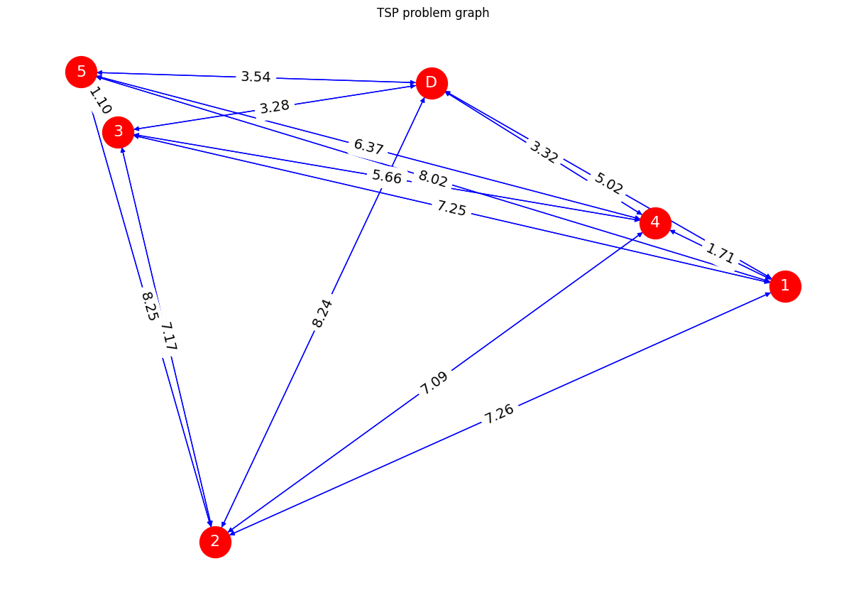
座標
D: [3.74540119 9.50714306]
1: [7.31993942 5.98658484]
2: [1.5601864 1.5599452]
3: [0.58083612 8.66176146]
4: [6.01115012 7.08072578]
5: [0.20584494 9.69909852]
距離行列
 [[0.         5.01713601 8.24215491 3.27553692 3.31980708 3.54475744]
 [5.01713601 0.         7.2642889  7.25066088 1.70589385 8.02453102]
 [8.24215491 7.2642889  0.         7.16902511 7.09155104 8.25106402]
 [3.27553692 7.25066088 7.16902511 0.         5.65579207 1.10303516]
 [3.31980708 1.70589385 7.09155104 5.65579207 0.         6.36847266]
 [3.54475744 8.02453102 8.25106402 1.10303516 6.36847266 0.        ]]

 

グラフで表現してみます。

以下、コードです。

import networkx as nx

# ネットワークのグラフ化
G = nx.DiGraph()
for i in range(n+1):
    for j in range(n+1):
        if i != j:
            G.add_edge(i, j, weight=dist[i, j])

plt.figure(figsize=(12, 8))
pos = {i: points[i] for i in range(n+1)}
labels = {i: f"D" if i == 0 else str(i) for i in range(n+1)}
weights = nx.get_edge_attributes(G, 'weight')
nx.draw(
    G, 
    pos, 
    with_labels=True, 
    labels=labels, 
    node_size=1000, 
    node_color='red', 
    font_size=16, 
    font_color='white', 
    edge_color='blue')
nx.draw_networkx_edge_labels(
    G, 
    pos, 
    font_size=14, 
    edge_labels={
        (i, j): f"{w:.2f}" for (i, j), 
        w in weights.items()})
plt.title("TSP problem graph")
plt.show()

 

以下、実行結果です。

 

　　最適化

最適化問題をモデル化し最適解を求めます。

以下、コードです。

# モデルの作成
prob = pulp.LpProblem("TSP", pulp.LpMinimize)

# 決定変数の定義
x = pulp.LpVariable.dicts(
    "route", 
    ((i, j) for i in range(n+1) for j in range(n+1) if i != j),
    cat='Binary')

# 目的関数
prob += pulp.lpSum(
    x[i, j] * dist[i, j] for i in range(n+1) for j in range(n+1) if i != j
)

# 制約条件
for i in range(n+1):
    prob += pulp.lpSum(x[i, j] for j in range(n+1) if i != j) == 1  # 各点から1度だけ出る
    prob += pulp.lpSum(x[j, i] for j in range(n+1) if i != j) == 1  # 各点に1度だけ入る

# サブツアー除去制約
u = pulp.LpVariable.dicts("u", range(1, n+1), lowBound=0, upBound=n)
for i in range(1, n+1):
    for j in range(1, n+1):
        if i != j:
            prob += u[i] - u[j] + n * x[i, j] <= n - 1

# 問題を解く
prob.solve(pulp.PULP_CBC_CMD(msg=False))

# 結果の表示
print(f"最適な総移動距離: {pulp.value(prob.objective):.2f}")

 

以下、実行結果です。

最適な総移動距離: 24.11

 

最適化の結果から、最適ルートを取得します。

以下、コードです。

# 最適ルートの取得
route = [0]
while len(route) < n + 2:
    added = False
    for j in range(n+1):
        if j not in route and pulp.value(x[route[-1], j]) == 1:
            route.append(j)
            added = True
            break
    if not added:
        break
        
print("最適ルート:", route)

 

以下、実行結果です。

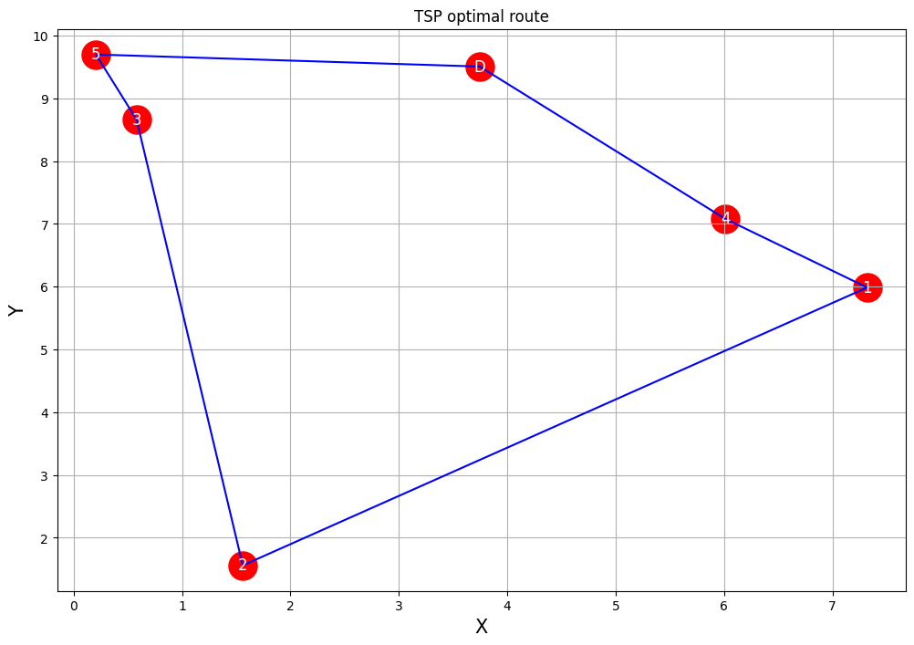
最適ルート: [0, 4, 1, 2, 3, 5]

 

グラフで表現してみます。

以下、コードです。

# 結果の可視化
plt.figure(figsize=(12, 8))
plt.scatter(points[:, 0], points[:, 1], c='red', s=500)
plt.plot(points[route + [0], 0], points[route + [0], 1], c='blue')
for i, point in enumerate(points):
    plt.annotate(
        f"{'D' if i == 0 else i}",
        (point[0], point[1]), 
        color='white', 
        fontsize=12,
        ha='center',  # フォントを真ん中寄せにする
        va='center'   # 垂直方向も真ん中寄せにする
    )
plt.title("TSP optimal route", fontsize=12)
plt.xlabel("X", fontsize=15)
plt.ylabel("Y", fontsize=15)
plt.grid(True)
plt.show()

 

以下、実行結果です。

 

これらのコードを実行すると、以下のことが分かります。

• 最適ルート: 各顧客をどの順序で訪問するべきかが分かります。
• 総移動距離: このルートで移動した場合の総距離が計算されます。

 

この結果から、以下のような洞察が得られます。

• 最も効率的な顧客訪問順序
• 総移動距離に基づく燃料コストや所要時間の見積もり

 

TSPは配送ルート最適化の基本ですが、現実の配送問題はより複雑です。そこで登場するのが、車両経路問題（VRP: Vehicle Routing Problem）です。

 

車両経路問題（VRP）

　問題設定

VRPは、TSPを拡張し、複数の車両や容量制約、時間枠制約などを考慮した問題です。

具体的には、どの車両に、どの顧客を割り当て、どのような順番で顧客を回ればいいのか、その最短ルートを求める問題です。

要は、顧客の割り当て問題と、最短ルート問題を解く問題です。

与えられた情報

• 配送車両：K台
• 各車両の容量
• 顧客数：n
• 各顧客の需要量
• 各顧客に時間枠制約（要望時間）
• 各顧客のサービス時間

目的

• 総移動距離を最小化しつつ、全ての制約を満たす配送計画を立てる

決定変数

• x_{ijk}: 車両kが地点iから地点jへ移動する場合は1、そうでない場合は0

制約条件

• 各顧客（地点）を1回だけ訪問すること
• 各車両はデポから出発し、デポに戻ってくること
• 車両の容量制約を守ること
• 顧客（地点）の時間枠制約を守ること
• 時間の連続性（到着時間が出発時間や移動時間、サービス時間などを考慮）を守ること
• 部分巡回（サブツアー）の除去

 

　数理モデル

　　モデル全体

車両経路問題（VRP）を定式化すると、以下のようになります。

\begin{array}{ll}\text{Minimize} \quad & \displaystyle \sum_{k=1}^{K} \sum_{i=0}^{n} \sum_{j=0, j \neq i}^{n} d_{ij} x_{ijk} \\ \text{subject to} \quad & \\ & \displaystyle \sum_{i=0}^{n} x_{i0k} = 1 \quad \forall k \in \{1, \ldots, K\} \\ & \displaystyle \sum_{j=0}^{n} x_{0jk} = 1 \quad \forall k \in \{1, \ldots, K\} \\ & \displaystyle \sum_{k=1}^{K} \sum_{j=0, j \neq i}^{n} x_{ijk} = 1 \quad \forall i \in \{0, 1, \ldots, n\} \\ & \displaystyle \sum_{k=1}^{K} \sum_{i=0, i \neq j}^{n} x_{ijk} = 1 \quad \forall j \in \{0, 1, \ldots, n\} \\ & \displaystyle \sum_{k=1}^{K} \sum_{i=0}^{n} q_i x_{ijk} \leq Q_k \quad \forall k \in \{1, \ldots, K\} \\[0.5cm] & \displaystyle a_i \leq t_{ik} \leq b_i \quad \forall k \in \{1, \ldots, K\}, \forall i \in \{0, 1, \ldots, n\} \\[0.3cm] & \displaystyle t_{jk} \geq t_{ik} + s_i + d_{ij} - M (1 - x_{ijk}) \quad \forall k \in \{1, \ldots, K\}, \forall i, j \in \{0, 1, \ldots, n\}, i \neq j \\[0.3cm] & \displaystyle x_{ijk} \in \{0, 1\} \quad \forall i, j \in \{0, 1, \ldots, n\}, \forall k \in \{1, \ldots, K\} \\[0.3cm] & \displaystyle t_{ik} \geq 0 \quad \forall i \in \{0, 1, \ldots, n\}, \forall k \in \{1, \ldots, K\}\\[0.3cm] & \displaystyle u_i - u_j + n x_{ijk} \leq n - 1 \quad \forall k \in \{1, \ldots, K\}, \forall i, j \in \{1, \ldots, n\}, i \neq j\end{array}

 

以下、変数です。

• x_{ijk} \in \{0, 1\}: 車両 k が地点 i から地点 j への移動を選択した場合に1、そうでない場合に0。
• t_{ik} \geq 0: 車両 k が地点 i に到着する時間。
• u_i \in \{0, 1, \ldots, n\}: 地点 i の順序を表す補助変数。

 

　　目的関数

総移動距離を最小化することを目的としています。

\displaystyle \text{Minimize} \quad \sum_{k=1}^{K} \sum_{i=0}^{n} \sum_{j=0, j \neq i}^{n} d_{ij} x_{ijk}

ここで、d_{ij} は地点 i から地点 j への距離を表し、x_{ijk} は車両 k が地点 i から地点 j への移動を選択した場合に1、そうでない場合に0となるバイナリ変数です。

 

　　制約条件

各車両はデポへ戻る

\displaystyle \sum_{i=0}^{n} x_{i0k} = 1 \quad \forall k \in \{1, \ldots, K\}

各車両 k は、デポに帰ってきます。ただし、1度だけです。

各車両はデポから出る

\displaystyle \sum_{j=0}^{n} x_{0jk} = 1 \quad \forall k \in \{1, \ldots, K\}

各車両 k は、デポから出発します。ただし、1度だけです。

いずれかの車両は各点（顧客）から1度だけ出る

\displaystyle \sum_{k=1}^{K} \sum_{j=0, j \neq i}^{n} x_{ijk} = 1 \quad \forall i \in \{0, 1, \ldots, n\}

各地点 i からは、他のいずれかの地点 j へ1度だけ移動する必要があります。

いずれかの車両は各点（顧客）に1度だけ入る

\displaystyle \sum_{k=1}^{K} \sum_{i=0, i \neq j}^{n} x_{ijk} = 1 \quad \forall j \in \{0, 1, \ldots, n\}

各地点 j には、他のいずれかの地点 i から1度だけ移動してくる必要があります。

車両の容量制約

\displaystyle \sum_{k=1}^{K} \sum_{i=0}^{n} q_i x_{ijk} \leq Q_k \quad \forall k \in \{1, \ldots, K\}

ここで、q_i は地点 i の需要量を表し、Q_k は車両 k の最大容量を表します。

時間枠制約

\displaystyle a_i \leq t_{ik} \leq b_i \quad \forall k \in \{1, \ldots, K\}, \forall i \in \{0, 1, \ldots, n\}

ここで、a_i と b_i は地点 i の時間枠の下限と上限を表し、t_{ik} は車両 k が地点 i に到着する時間を表します。

時間の連続性制約

\displaystyle t_{jk} \geq t_{ik} + s_i + d_{ij} - M (1 - x_{ijk}) \quad \forall k \in \{1, \ldots, K\}, \forall i, j \in \{0, 1, \ldots, n\}, i \neq j

ここで、s_i は地点 i でのサービス時間を表し、M は十分に大きな定数です。この制約は、車両が次の地点に移動するための時間を考慮しています。

サブツアー除去制約

\displaystyle u_i - u_j + n x_{ijk} \leq n - 1 \quad \forall k \in \{1, \ldots, K\}, \forall i, j \in \{1, \ldots, n\}, i \neq j

この制約は、サブツアー（部分的な巡回路）が発生しないようにするためのものです。u_i は補助変数で、地点 i の順序を表します。

 

　Pythonによる実装

VRPを解くために、OR-Toolsライブラリを使用します。OR-Toolsは、Googleが開発した最適化ソルバーで、VRPのような複雑な問題を効率的に解くことができます。

 

　　必要なモジュールの読み込み

まず、必要なモジュールを読み込みます。

以下、コードです。

# 必要なライブラリのインポート
from ortools.constraint_solver import routing_enums_pb2
from ortools.constraint_solver import pywrapcp
import numpy as np
import matplotlib.pyplot as plt

 

車両経路問題（VRP: Vehicle Routing Problem）を解くために以下をインポートします。

from ortools.constraint_solver import routing_enums_pb2

• ルーティングアルゴリズムの動作を制御するための定数を定義するためのものです。
• 具体的には、初期解法戦略や局所探索のメタヒューリスティックなどのアルゴリズムを設定するのに利用します。
• 初期解法戦略とは、ルーティング問題の初期解を生成するための方法のことです。
• 局所探索のメタヒューリスティックとは、初期解を改善するための探索アルゴリズムのことです。

from ortools.constraint_solver import pywrapcp

• ルーティングモデルやインデックスマネージャーなど、ルーティング問題を解くためのクラスや関数です。
• ルーティングモデルは、ルーティング問題の定式化と解法を管理するためのクラスです。
• インデックスマネージャーは、ルーティングモデル内で使用されるノードのインデックスを管理するためのクラスです。
• これらのコンポーネントを組み合わせ、ルーティング問題を定式化し解きます。

 

インデックスマネージャーとルーティングモデルのインスタンスを生成し、VRPの定式化などの設定を行います。

それをどのように解くのかを、初期解法戦略や局所探索のメタヒューリスティックなどのアルゴリズムを設定し、問題を解いていきます。

 

　　サンプルデータの生成

次に、サンプルデータを生成します。

このサンプルデータのデータモデルの構成要素は以下の通りです。

• num_vehicles: 車両数
• depot: デポ（出発地点）のインデックス
• locations: 各地点の座標（デポを含む）
• demands: 各地点の需要量（デポの需要は0）
• vehicle_capacities: 各車両の容量
• service_times: 各顧客のサービス時間
• time_windows: 各地点の時間枠
• distance_matrix: 各地点間の距離行列

 

では、生成します。サンプルデータは辞書型（dictionary）で格納します。

以下、コードです。

# データモデルの作成
def create_data_model():
    """問題のデータを格納します。"""
    data = {}
    data['num_vehicles'] = 3  # 車両数
    data['depot'] = 0
    # 10顧客 + デポのためのランダムな座標を生成
    np.random.seed(42)
    data['locations'] = np.random.rand(11, 2) * 100
    # ランダムな需要を生成
    data['demands'] = np.random.randint(1, 4, 11) 
    data['demands'][0] = 0  # デポの需要は0
    # ランダムな車両容量を生成
    data['vehicle_capacities'] = np.random.randint(10, 20, data['num_vehicles'])
    # 顧客のサービス時間を設定（例: 一律10分）
    data['service_times'] = np.full(11, 10)
    data['service_times'][0] = 0  # デポのサービス時間は0
    # 時間枠を生成
    data['time_windows'] = [(0, 2000)] + [(np.random.randint(0, 200), np.random.randint(801, 2000)) for _ in range(10)]
    # 距離行列を計算
    data['distance_matrix'] = (np.sqrt(((data['locations'][:, None, :] - data['locations'][None, :, :]) ** 2).sum(axis=-1)) * 10).astype(int)
    return data

# データモデルを作成
data = create_data_model()

# 確認用の出力
print("Vehicle capacities:", data['vehicle_capacities'])
print("Customer demands:", data['demands'])
print("Service times:", data['service_times'])
print("Time windows:", data['time_windows'])

 

以下、実行結果です。

Vehicle capacities: [16 14 18]
Customer demands: [0 2 2 3 2 3 3 1 3 1 3]
Service times: [ 0 10 10 10 10 10 10 10 10 10 10]
Time windows: [(0, 2000), (166, 1188), (88, 1116), (13, 1042), (8, 1365), (129, 892), (110, 1756), (198, 1309), (7, 835), (80, 1826), (133, 1366)]

 

グラフで表現してみます。

以下、コードです。

import networkx as nx

# データモデルの取得
locations = data['locations']
distance_matrix = data['distance_matrix']

# グラフの作成
G = nx.DiGraph()
for i in range(len(locations)):
    for j in range(len(locations)):
        if i != j:
            G.add_edge(i, j, weight=distance_matrix[i, j])

# グラフの描画
plt.figure(figsize=(12, 8))
pos = {i: locations[i] for i in range(len(locations))}
labels = {i: f"D" if i == 0 else str(i) for i in range(len(locations))}
weights = nx.get_edge_attributes(G, 'weight')
nx.draw(
    G, 
    pos, 
    with_labels=True, 
    labels=labels, 
    node_size=1000, 
    node_color='red', 
    font_size=16, 
    font_color='white', 
    edge_color='blue')
nx.draw_networkx_edge_labels(
    G, 
    pos, 
    font_size=14, 
    edge_labels={
        (i, j): f"{w:.2f}" for (i, j), 
        w in weights.items()})
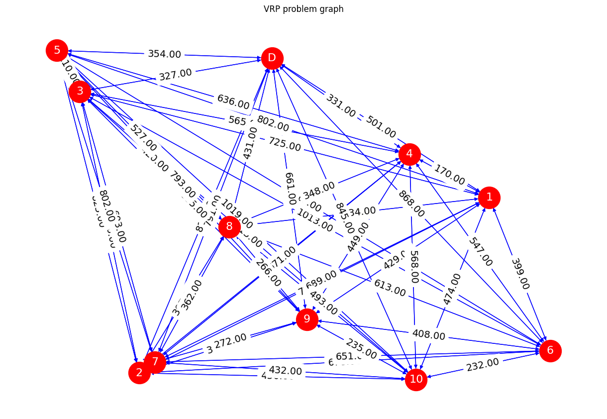
plt.title("VRP problem graph")
plt.show()

 

以下、実行結果です。

 

　　最適化

車両経路問題（VRP: Vehicle Routing Problem）を解くための準備を行います。

以下、コードです。

if solution:
    plt.figure(figsize=(12, 8))
    plt.scatter(data['locations'][:, 0], data['locations'][:, 1], c='red', s=500)
    plt.scatter(data['locations'][0, 0], data['locations'][0, 1], c='green', s=100, marker='s') 
    for i, coord in enumerate(data['locations']):
        plt.annotate(
            str(i), 
            (coord[0], coord[1]), 
            fontsize=12, 
            color='white', 
            ha='center',  # フォントを真ん中寄せにする
            va='center'   # 垂直方向も真ん中寄せにする
        )
    
    colors = ['b', 'g', 'r', 'c', 'm', 'y', 'k', 'orange']
    for vehicle_id in range(data['num_vehicles']):
        index = routing.Start(vehicle_id)
        route = []
        while not routing.IsEnd(index):
            node_index = manager.IndexToNode(index)
            route.append(node_index)
            index = solution.Value(routing.NextVar(index))
        route.append(manager.IndexToNode(index))
        
        route_coords = data['locations'][route]
        plt.plot(
            route_coords[:, 0], 
            route_coords[:, 1], 
            c=colors[vehicle_id % len(colors)], 
            linewidth=2, label=f'Vehicle {vehicle_id}')
    
    plt.title('VRP Solution')
    plt.xlabel('X')
    plt.ylabel('Y')
    plt.legend()
    plt.grid(True)
    plt.show()
else:
    print('No solution to visualize.')

 

コードを簡単に説明します。

ルーティングインデックスマネージャーとモデルの作成

• RoutingIndexManager
  • ノード（地点）と車両のインデックスを管理するためのクラスです。
  • これにより、ユーザーが定義したノードのインデックスと、ルーティングモデル内で使用される内部インデックスを相互に変換することができます。
• RoutingModel
  • ルーティング問題の定式化と解法を管理するためのクラスです。
  • 具体的には、ノード間の移動コスト、制約条件（例えば、車両の容量や時間枠）、および目的関数（例えば、総移動距離の最小化）を定義します。

距離コールバックの追加

• distance_callback関数は、2つのノード間の距離を計算して返す関数です。
• この関数は、ルーティングモデルに登録され、各車両の移動コスト（距離）を計算するために使用されます。

容量制約の追加

• demand_callback関数は、各ノードの需要量を計算して返す関数です。
• この関数は、ルーティングモデルに登録され、各車両の容量制約を追加するために使用されます。
• これにより、各車両がその容量を超えないように制約が追加されます。

時間枠制約の追加

• time_callback関数は、2つのノード間の移動時間を計算して返す関数です。
• この関数は、ルーティングモデルに登録され、各車両の時間枠制約を追加するために使用されます。
• 各ノードの時間枠を設定することで、特定の時間内に訪問する必要があるように制約が追加され、現実的なスケジュールを考慮したルートが生成されます。
• これにより、車両経路問題を解くための準備が整いました。次のステップでは、探索パラメータを設定し、問題を解くことができます。

 

車両経路問題（VRP: Vehicle Routing Problem）を解きます。

以下、コードです。

# 初期解法の設定
search_parameters = pywrapcp.DefaultRoutingSearchParameters()
search_parameters.first_solution_strategy = (
    routing_enums_pb2.FirstSolutionStrategy.AUTOMATIC)
search_parameters.local_search_metaheuristic = (
    routing_enums_pb2.LocalSearchMetaheuristic.GUIDED_LOCAL_SEARCH)
search_parameters.time_limit.FromSeconds(180) 

# 問題を解く
solution = routing.SolveWithParameters(search_parameters)

 

このコードで、車両経路問題（VRP: Vehicle Routing Problem）を解くための探索パラメータを設定し、問題を解きます。

初期解法の設定

• search_parametersのインスタンスを作成します。
• first_solution_strategyをAUTOMATICに設定します。これは、初期解法の戦略を自動的に選択することを意味します。
• local_search_metaheuristicをGUIDED_LOCAL_SEARCHに設定します。これは、局所探索のメタヒューリスティックとしてガイド付き局所探索アルゴリズムを使用することを意味します。
• time_limitを180秒に設定します。これは、探索にかける最大時間を180秒に制限することを意味します。

問題を解く

• routing.SolveWithParametersメソッドを使用して、設定した探索パラメータで車両経路問題を解きます。
• 解が見つかった場合、solutionに解が格納されます。

 

では、解を表示します。

以下、コードです。

# 解の表示
if solution:
    total_distance = 0
    total_load = 0
    for vehicle_id in range(data['num_vehicles']):
        index = routing.Start(vehicle_id)
        plan_output = f'Route for vehicle {vehicle_id}:\n'
        route_distance = 0
        route_load = 0
        while not routing.IsEnd(index):
            node_index = manager.IndexToNode(index)
            route_load += data['demands'][node_index]
            plan_output += f' {node_index} Load({route_load}) -> '
            previous_index = index
            index = solution.Value(routing.NextVar(index))
            route_distance += routing.GetArcCostForVehicle(previous_index, index, vehicle_id)
        plan_output += f' {manager.IndexToNode(index)} Load({route_load})\n'
        plan_output += f'Distance of the route: {route_distance}m\n'
        plan_output += f'Load of the route: {route_load}\n'
        print(plan_output)
        total_distance += route_distance
        total_load += route_load
    print(f'Total distance of all routes: {total_distance}m')
    print(f'Total load of all routes: {total_load}')
else:
    print('No solution found !')

 

以下、実行結果です。

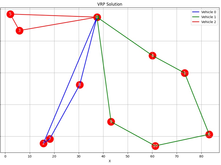
Route for vehicle 0:
 0 Load(0) ->  8 Load(3) ->  7 Load(4) ->  2 Load(6) ->  0 Load(6)
Distance of the route: 1654m
Load of the route: 6

Route for vehicle 1:
 0 Load(0) ->  4 Load(2) ->  1 Load(4) ->  6 Load(7) ->  10 Load(10) ->  9 Load(11) ->  0 Load(11)
Distance of the route: 2028m
Load of the route: 11

Route for vehicle 2:
 0 Load(0) ->  3 Load(3) ->  5 Load(6) ->  0 Load(6)
Distance of the route: 791m
Load of the route: 6

Total distance of all routes: 4473m
Total load of all routes: 23

 

グラフで表現してみます。

以下、コードです。

if solution:
    plt.figure(figsize=(12, 8))
    plt.scatter(data['locations'][:, 0], data['locations'][:, 1], c='red', s=500)
    plt.scatter(data['locations'][0, 0], data['locations'][0, 1], c='green', s=100, marker='s') 
    for i, coord in enumerate(data['locations']):
        plt.annotate(
            str(i), 
            (coord[0], coord[1]), 
            fontsize=12, 
            color='white', 
            ha='center',  # フォントを真ん中寄せにする
            va='center'   # 垂直方向も真ん中寄せにする
        )
    
    colors = ['b', 'g', 'r', 'c', 'm', 'y', 'k', 'orange']
    for vehicle_id in range(data['num_vehicles']):
        index = routing.Start(vehicle_id)
        route = []
        while not routing.IsEnd(index):
            node_index = manager.IndexToNode(index)
            route.append(node_index)
            index = solution.Value(routing.NextVar(index))
        route.append(manager.IndexToNode(index))
        
        route_coords = data['locations'][route]
        plt.plot(
            route_coords[:, 0], 
            route_coords[:, 1], 
            c=colors[vehicle_id % len(colors)], 
            linewidth=2, label=f'Vehicle {vehicle_id}')
    
    plt.title('VRP Solution')
    plt.xlabel('X')
    plt.ylabel('Y')
    plt.legend()
    plt.grid(True)
    plt.show()
else:
    print('No solution to visualize.')

 

以下、実行結果です。

 

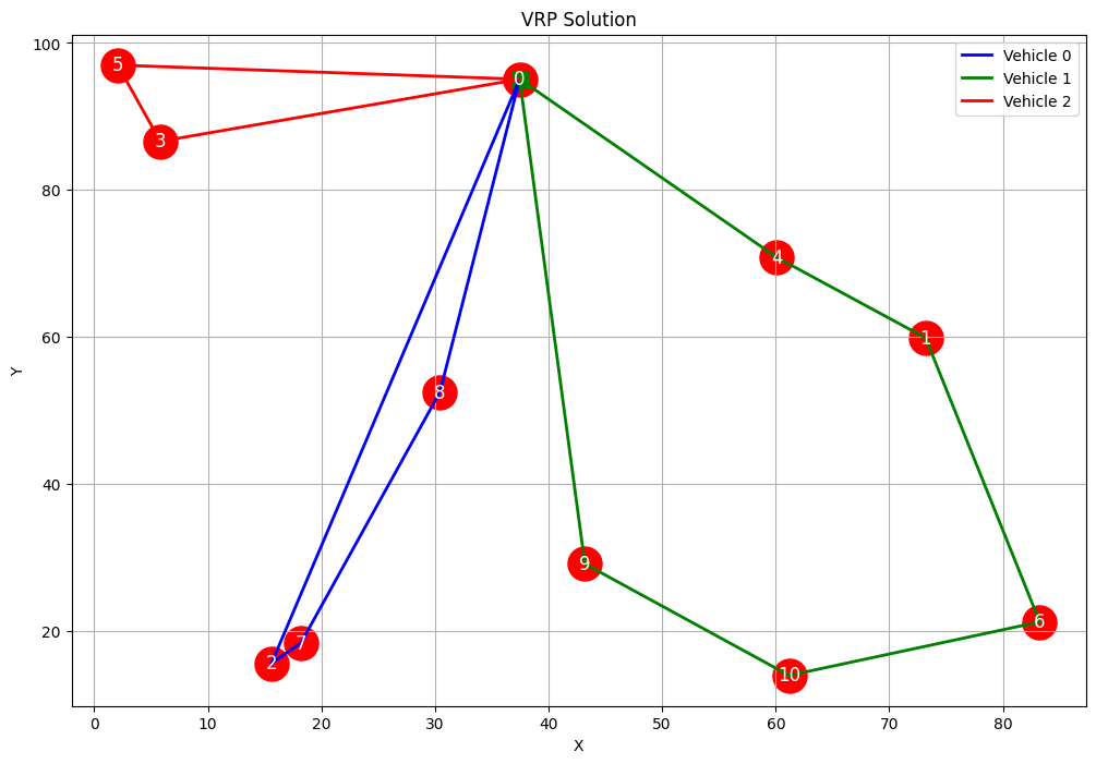
これらのコードを実行すると、以下のことが分かります。

• 各車両のルート：どの車両がどの顧客を訪問するかが分かります。
• ルートごとの距離と負荷：各車両の移動距離と積載量が計算されます。
• 総距離と総負荷：全車両の合計移動距離と合計積載量が示されます。

 

この結果から、以下のような洞察が得られます。

• 各車両の効率的な顧客訪問順序
• 車両ごとの負荷バランス
• 時間枠制約の遵守状況

 

要は、このようなVRPの解は、以下のような実務的な意思決定に活用できます。

• 配送計画の最適化：各車両の効率的なルートを決定
• 車両の適切な配置：需要に応じた車両の割り当て
• 人員配置の最適化：ドライバーのシフト計画への反映
• 顧客サービスの向上：時間枠遵守による顧客満足度の向上
• コスト削減：燃料費や人件費の最小化

 

より発展した話題

ここまで、配送ルート最適化の基本的な問題であるTSPから、より現実的なVRPまでを扱いました。

配送ルート最適化は、以下のような発展版があります。

• 動的VRP：リアルタイムの交通情報や新規注文を考慮した動的な経路計画
• グリーンVRP：CO2排出量を考慮した環境に配慮した経路最適化
• 確率的VRP：需要や移動時間の不確実性を考慮したロバストな計画
• マルチデポVRP：複数の倉庫を考慮した大規模な配送網の最適化
• ドローン配送との統合：トラックとドローンを組み合わせたハイブリッド配送の最適化

 

ただ、実務での活用に向けては、以下の点に注意が必要です。

• データの質と精度の向上：正確な距離データ、需要予測、時間見積もりの重要性
• システム統合：既存の配送管理システムとの連携
• ユーザーインターフェースの開発：計画立案者が使いやすいツールの設計
• リアルタイムモニタリングと再最適化：予期せぬ事態への対応
• ドライバーとの協調：最適化結果の現場での受け入れと活用

 

配送ルート最適化は、物流コストの削減、顧客サービスの向上、環境負荷の低減など、多面的な効果をもたらします。

今回取り上げたアプローチを基礎として、より複雑な現実世界の問題に取り組むことで、効率的で持続可能な物流オペレーションの実現に貢献できるでしょう。

数学的な厳密性と現場の現実をバランスよく考慮し、継続的に改善を重ねることが、成功への鍵となります。

 

まとめ

今回は、Pythonを用いた配送ルート最適化の基本的な概念から実践的な実装まで、段階的にお話ししました。

まず、最も基本的な巡回セールスマン問題（TSP）を通じて、単一の車両が全ての顧客を訪問する最適ルートを求める方法をお話ししました。PuLPライブラリを使用してTSPを数理モデル化し、最適解を得る過程を詳しく見ていきました。

次に、より現実的な制約を考慮した車両経路問題（VRP）へと発展させ、複数の車両、容量制約、時間枠制約などを含む複雑な問題の解法を説明しました。VRPの解法にはOR-Toolsライブラリを活用し、大規模かつ複雑な最適化問題に対処する方法を示しました。

このような最適化アプローチは、物流コストの削減、顧客サービスの向上、環境負荷の低減など、多面的な効果をもたらす可能性があります。

数理最適化とPythonプログラミングのスキルを組み合わせることで、読者は実際のビジネス課題に対して効果的なソリューションを提供できるようになるでしょう。