次の Python コードの出力はどれでしょうか？

Python コード:

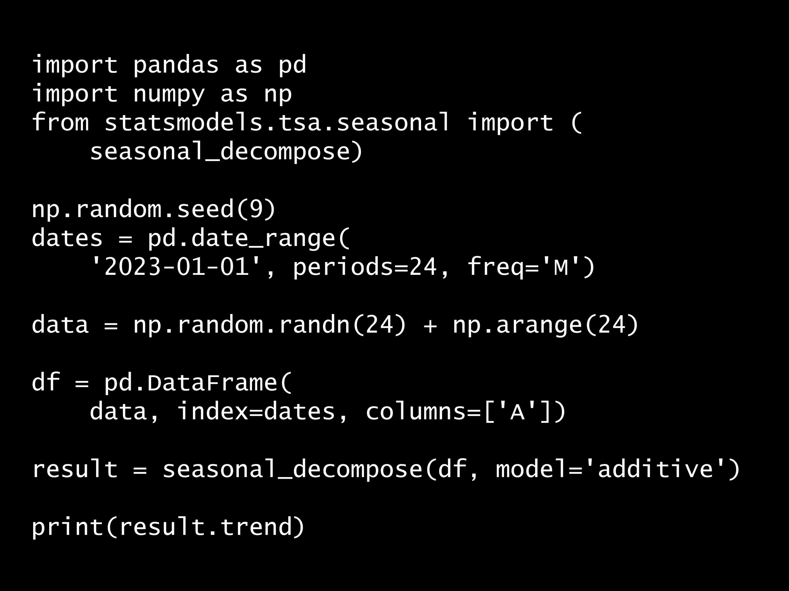
import pandas as pd
import numpy as np
from statsmodels.tsa.seasonal import seasonal_decompose

np.random.seed(9)
dates = pd.date_range(
    '2023-01-01', 
    periods=24,  # increase the period to 24
    freq='M')
data = np.random.randn(24) + np.arange(24)
df = pd.DataFrame(
    data, 
    index=dates, 
    columns=['A'])
result = seasonal_decompose(df, model='additive')

print(result.trend)

回答の選択肢:

(A) ランダムな値
(B) 各月のトレンドの値
(C) 各月の値からトレンドを引いた値
(D) 各月の値から季節成分を引いた値

出力例:

2023-01-31          NaN
2023-02-28          NaN
2023-03-31          NaN
2023-04-30          NaN
2023-05-31          NaN
2023-06-30          NaN
2023-07-31     5.779174
2023-08-31     6.833033
2023-09-30     7.997030
2023-10-31     9.137969
2023-11-30    10.236500
2023-12-31    11.299062
2024-01-31    12.339088
2024-02-29    13.471116
2024-03-31    14.583799
2024-04-30    15.650293
2024-05-31    16.690383
2024-06-30    17.645493
2024-07-31          NaN
2024-08-31          NaN
2024-09-30          NaN
2024-10-31          NaN
2024-11-30          NaN
2024-12-31          NaN
Freq: M, Name: trend, dtype: float64

正解:

(B)

解説:

このコードは、時間の経過と共に増加するトレンドを持つ時系列データを作成し、それを季節性分解によってトレンド部分と残りに分けています。

詳しく説明します。

‘2023-01-01’から始まる月単位の日付範囲を24期間作成します。

dates = pd.date_range(
    '2023-01-01', 
    periods=24,
    freq='M')

datesに格納されているデータは次のようになっています。

DatetimeIndex(['2023-01-31', '2023-02-28', '2023-03-31', '2023-04-30',
               '2023-05-31', '2023-06-30', '2023-07-31', '2023-08-31',
               '2023-09-30', '2023-10-31', '2023-11-30', '2023-12-31',
               '2024-01-31', '2024-02-29', '2024-03-31', '2024-04-30',
               '2024-05-31', '2024-06-30', '2024-07-31', '2024-08-31',
               '2024-09-30', '2024-10-31', '2024-11-30', '2024-12-31'],
              dtype='datetime64[ns]', freq='M')

ランダムな正規分布に従うデータに、増加する連続数列を加えることで、時間の経過と共に増加するトレンドを持つデータセットを生成します。

data = np.random.randn(24) + np.arange(24)

dataに格納されているデータは次のようになっています。

[1.10855471e-03 7.10455931e-01 8.83933697e-01 2.98711724e+00
 3.62163854e+00 4.51886464e+00 4.48266882e+00 6.50912802e+00
 7.75931942e+00 8.35205254e+00 1.06358911e+01 1.27401173e+01
 1.22966822e+01 1.37075037e+01 1.58228158e+01 1.54307690e+01
 1.75427296e+01 1.60992788e+01 1.78628750e+01 2.02975790e+01
 2.06752712e+01 2.10319581e+01 2.29181459e+01 2.33805095e+01]

このデータを日付範囲をインデックスにしたデータフレームに格納します。このデータフレームの列名は ‘A’ です。

df = pd.DataFrame(
    data, 
    index=dates, 
    columns=['A'])

dfに格納されているデータは次のようになっています。

                    A
2023-01-31   0.001109
2023-02-28   0.710456
2023-03-31   0.883934
2023-04-30   2.987117
2023-05-31   3.621639
2023-06-30   4.518865
2023-07-31   4.482669
2023-08-31   6.509128
2023-09-30   7.759319
2023-10-31   8.352053
2023-11-30  10.635891
2023-12-31  12.740117
2024-01-31  12.296682
2024-02-29  13.707504
2024-03-31  15.822816
2024-04-30  15.430769
2024-05-31  17.542730
2024-06-30  16.099279
2024-07-31  17.862875
2024-08-31  20.297579
2024-09-30  20.675271
2024-10-31  21.031958
2024-11-30  22.918146
2024-12-31  23.380509

`seasonal_decompose`関数を使用して時系列データをトレンド、季節性、残差に分解します。ここでは加法モデル(`model=’additive’`)を使用しています。加法モデルでは、時系列データはトレンド、季節性、残差の和として表されます。

result = seasonal_decompose(df, model='additive')

`result`オブジェクトは、時系列データを季節性分解した結果を保持しています。

これにはトレンド（`result.trend`）、季節性（`result.seasonal`）、残差（`result.resid`）、観測された元のデータ（`result.observed`）の4つの主要な成分が含まれます。これらの各成分は、元のデータの同じ時間インデックスを持つpandasのSeriesです。

• `result.trend`：データの底流するトレンドを示します。これはデータの長期的な進行方向を示しています。
• `result.seasonal`：データの季節性パターンを示します。これは一年を通じての周期的な変動または他の既知の周期を示しています。
• `result.resid`：トレンドと季節性によって説明されないデータの変動を示します。これはデータ内のランダムなノイズを示しています。
• `result.observed`：観測された原始のデータを示します。

最後に、この分解結果からトレンド成分を取り出して表示します。

print(result.trend)

ただし、この結果には、移動平均の計算に必要なデータが不足している始めと終わりの期間に対するNaN（非数）が含まれています。

2023-01-31          NaN
2023-02-28          NaN
2023-03-31          NaN
2023-04-30          NaN
2023-05-31          NaN
2023-06-30          NaN
2023-07-31     5.779174
2023-08-31     6.833033
2023-09-30     7.997030
2023-10-31     9.137969
2023-11-30    10.236500
2023-12-31    11.299062
2024-01-31    12.339088
2024-02-29    13.471116
2024-03-31    14.583799
2024-04-30    15.650293
2024-05-31    16.690383
2024-06-30    17.645493
2024-07-31          NaN
2024-08-31          NaN
2024-09-30          NaN
2024-10-31          NaN
2024-11-30          NaN
2024-12-31          NaN
Freq: M, Name: trend, dtype: float64

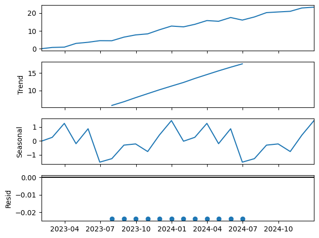
ちなみに、各成分は `result.plot()` を使用して視覚的に描画することができます。

import matplotlib.pyplot as plt

result.plot()
plt.show()

Python 時系列分析 1,000本ノック– ノック20: 時系列データの変数変換 –