Python 時系列分析 1,000本ノック– ノック68: 状態空間モデルの推定 –

問題
答え
解説

次の Python コードで推定しているのは何ですか？

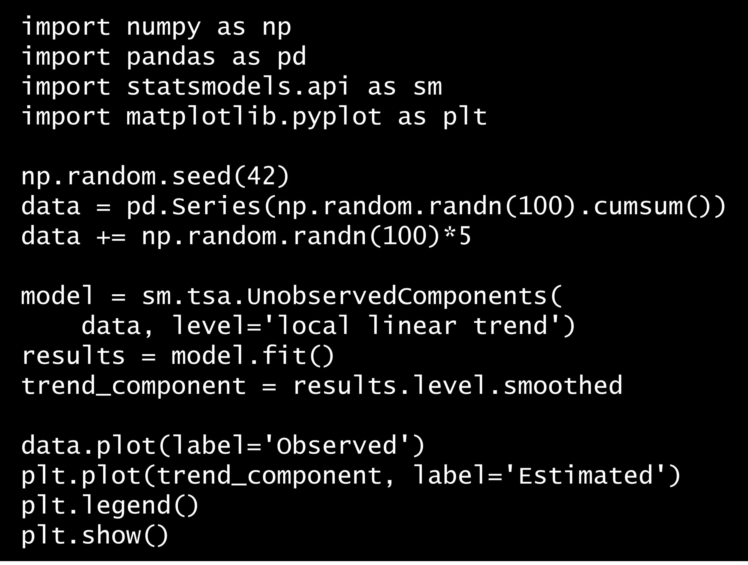
Python コード:

import numpy as np

import pandas as pd

import statsmodels.api as sm

import matplotlib.pyplot as plt

np.random.seed(42)

data = pd.Series(np.random.randn(100).cumsum())

data += np.random.randn(100)*5

model = sm.tsa.UnobservedComponents(

data, level='local linear trend')

results = model.fit()

trend_component = results.level.smoothed

data.plot(label='Observed')

plt.plot(trend_component, label='Estimated')

plt.legend()

plt.show()

import numpy as np import pandas as pd import statsmodels.api as sm import matplotlib.pyplot as plt np.random.seed(42) data = pd.Series(np.random.randn(100).cumsum()) data += np.random.randn(100)*5 model = sm.tsa.UnobservedComponents( data, level='local linear trend') results = model.fit() trend_component = results.level.smoothed data.plot(label='Observed') plt.plot(trend_component, label='Estimated') plt.legend() plt.show()

import numpy as np
import pandas as pd
import statsmodels.api as sm
import matplotlib.pyplot as plt

np.random.seed(42)
data = pd.Series(np.random.randn(100).cumsum())
data += np.random.randn(100)*5

model = sm.tsa.UnobservedComponents(
    data, level='local linear trend')
results = model.fit()
trend_component = results.level.smoothed

data.plot(label='Observed')
plt.plot(trend_component, label='Estimated')
plt.legend()
plt.show()

回答の選択肢:

(A) ノイズ成分
(B) 長期的な変動
(C) 短期的な変動
(D) 季節成分

出力例:

RUNNING THE L-BFGS-B CODE

           * * *

Machine precision = 2.220D-16
 N =            3     M =           10

At X0         0 variables are exactly at the bounds

At iterate    0    f=  3.45332D+00    |proj g|=  5.68564D-02

At iterate    5    f=  3.07868D+00    |proj g|=  8.58802D-03

At iterate   10    f=  3.07821D+00    |proj g|=  1.10342D-04

At iterate   15    f=  3.07817D+00    |proj g|=  4.95151D-03

At iterate   20    f=  3.07816D+00    |proj g|=  2.92184D-05

           * * *

Tit   = total number of iterations
Tnf   = total number of function evaluations
Tnint = total number of segments explored during Cauchy searches
Skip  = number of BFGS updates skipped
Nact  = number of active bounds at final generalized Cauchy point
Projg = norm of the final projected gradient
F     = final function value

           * * *

   N    Tit     Tnf  Tnint  Skip  Nact     Projg        F
    3     21     34      1     0     0   2.120D-06   3.078D+00
  F =   3.0781566397632201     

CONVERGENCE: NORM_OF_PROJECTED_GRADIENT_<=_PGTOL            
 This problem is unconstrained.

正解: (B)

回答の選択肢:

(A) ノイズ成分
(B) 長期的な変動
(C) 短期的な変動
(D) 季節成分

コードの解説

このコードは、時系列データの長期的な変動（トレンド）を推定するために、statsmodelsライブラリのUnobservedComponentsモデルを使用しています。

import numpy as np

import pandas as pd

import statsmodels.api as sm

import matplotlib.pyplot as plt

np.random.seed(42)

data = pd.Series(np.random.randn(100).cumsum())

data += np.random.randn(100)*5

model = sm.tsa.UnobservedComponents(

data, level='local linear trend')

results = model.fit()

trend_component = results.level.smoothed

data.plot(label='Observed')

plt.plot(trend_component, label='Estimated')

plt.legend()

plt.show()

import numpy as np
import pandas as pd
import statsmodels.api as sm
import matplotlib.pyplot as plt

np.random.seed(42)
data = pd.Series(np.random.randn(100).cumsum())
data += np.random.randn(100)*5

model = sm.tsa.UnobservedComponents(
    data, level='local linear trend')
results = model.fit()
trend_component = results.level.smoothed

data.plot(label='Observed')
plt.plot(trend_component, label='Estimated')
plt.legend()
plt.show()

詳しく説明します。

data という名前のpandas.Seriesを作成し、ランダムウォーク（累積和）にノイズを加えたデータを生成します。

np.random.seed(42)

data = pd.Series(np.random.randn(100).cumsum())

data += np.random.randn(100)*5

np.random.seed(42) data = pd.Series(np.random.randn(100).cumsum()) data += np.random.randn(100)*5

np.random.seed(42)
data = pd.Series(np.random.randn(100).cumsum())
data += np.random.randn(100)*5

data には、以下のようなデータが格納されています。

0     -6.580140
1     -1.744777
2     -0.707434
3     -1.482218
4      1.488586
        ...    
95    -8.785767
96   -14.835521
97    -9.386553
98    -9.859021
99   -16.099503
Length: 100, dtype: float64

UnobservedComponentsを使用して、データに対して「ローカル線形トレンド」モデルを定義します。model.fit()を呼び出してモデルをデータにフィットさせ、結果をresultsに格納します。

model = sm.tsa.UnobservedComponents(

data, level='local linear trend')

results = model.fit()

model = sm.tsa.UnobservedComponents( data, level='local linear trend') results = model.fit()

model = sm.tsa.UnobservedComponents(
    data, level='local linear trend')
results = model.fit()

results.level.smoothedを使用して、推定されたトレンド成分を抽出し、trend_componentに格納します。

trend_component = results.level.smoothed

trend_component = results.level.smoothed

元の観測データと推定されたトレンド成分をプロットし、視覚的に比較します。

data.plot(label='Observed')

plt.plot(trend_component, label='Estimated')

plt.legend()

plt.show()

data.plot(label='Observed') plt.plot(trend_component, label='Estimated') plt.legend() plt.show()

data.plot(label='Observed')
plt.plot(trend_component, label='Estimated')
plt.legend()
plt.show()

RUNNING THE L-BFGS-B CODE

           * * *

Machine precision = 2.220D-16
 N =            3     M =           10

At X0         0 variables are exactly at the bounds

At iterate    0    f=  3.45332D+00    |proj g|=  5.68564D-02

At iterate    5    f=  3.07868D+00    |proj g|=  8.58802D-03

At iterate   10    f=  3.07821D+00    |proj g|=  1.10342D-04

At iterate   15    f=  3.07817D+00    |proj g|=  4.95151D-03

At iterate   20    f=  3.07816D+00    |proj g|=  2.92184D-05

           * * *

Tit   = total number of iterations
Tnf   = total number of function evaluations
Tnint = total number of segments explored during Cauchy searches
Skip  = number of BFGS updates skipped
Nact  = number of active bounds at final generalized Cauchy point
Projg = norm of the final projected gradient
F     = final function value

           * * *

   N    Tit     Tnf  Tnint  Skip  Nact     Projg        F
    3     21     34      1     0     0   2.120D-06   3.078D+00
  F =   3.0781566397632201     

CONVERGENCE: NORM_OF_PROJECTED_GRADIENT_<=_PGTOL            
 This problem is unconstrained.

状態空間モデルとstatsmodels

Contents [hide]

状態空間モデルの基礎
基本的な状態空間モデル
　ローカルレベルモデル（Local Level Model）
　ローカル線形トレンドモデル（Local Linear Trend Model）
　季節性モデル（Seasonal Model）
statsmodelsを使用した状態空間モデルの実装
簡単な時系列データの分析例

状態空間モデルの基礎

状態空間モデルは、時系列データ分析において非常に強力かつ柔軟なツールです。このモデルは、観測可能なデータと直接観測できない潜在的な状態の両方を考慮することができ、経済予測、信号処理、制御工学、生態学など、様々な分野で広く応用されています。

状態空間モデルの主な特徴は以下です。

潜在状態の考慮: 直接観測できない潜在的な状態（状態変数）を扱います。
時間変化: 時間とともに変化する状態を表現できます。
柔軟性: 複雑な時系列データの構造を柔軟にモデル化できます。
ノイズの明示的取り扱い: プロセスノイズと観測ノイズを明示的にモデル化します。

状態空間モデルは以下のような場面で特に有用です。

トレンドや季節性が時間とともに変化する時系列データの分析
ノイズの多いデータからの信号抽出
複数の要因が絡み合う複雑なシステムのモデリング
欠損データを含む時系列の処理

状態空間モデルは通常、以下の2つの方程式で表現されます。

状態方程式（遷移方程式）:

\displaystyle x_t = F_t x_{t-1} + w_t

観測方程式:

\displaystyle y_t = H_t x_t + v_t

ここで、

$x_t$ : 時刻tでの状態ベクトル
$y_t$ : 時刻tでの観測ベクトル
$F_t$ : 状態遷移行列
$H_t$ : 観測行列
$w_t$ : プロセスノイズ（通常、正規分布を仮定）
$v_t$ : 観測ノイズ（通常、正規分布を仮定）

この表現は、システムの動的な性質（状態方程式）と、その状態が観測値にどのように反映されるか（観測方程式）を明示的に示しています。

基本的な状態空間モデル

ここでは、代表的な基本的状態空間モデルを紹介します。

　ローカルレベルモデル（Local Level Model）

ローカルレベルモデル（別名：ランダムウォークプラスノイズモデル）は、最も単純な状態空間モデルの一つです。

状態方程式：

\displaystyle \mu_t = \mu_{t-1} + \eta_t

観測方程式：

\displaystyle y_t = \mu_t + \varepsilon_t

ここで、

$\mu_t$ : 時刻tでの状態（レベル）
$y_t$ : 時刻tでの観測値
$\eta_t \sim N(0, \sigma_\eta^2)$ : レベルのノイズ
$\varepsilon_t \sim N(0, \sigma_\varepsilon^2)$ : 観測ノイズ

このモデルは、時間とともにランダムに変動するレベル（平均）を持つ時系列データに適しています。例えば、株価や為替レートなどの金融データ、あるいは気温データなどの環境データの分析に使用されることがあります。

　ローカル線形トレンドモデル（Local Linear Trend Model）

ローカル線形トレンドモデルは、ローカルレベルモデルを拡張し、トレンド（傾き）を含めたモデルです。

レベルの方程式：

\displaystyle \mu_t = \mu_{t-1} + \nu_{t-1} + \eta_t

トレンドの方程式：

\displaystyle \nu_t = \nu_{t-1} + \zeta_t

観測方程式：

\displaystyle y_t = \mu_t + \varepsilon_t

ここで、

$\mu_t$ : 時刻tでのレベル
$\nu_t$ : 時刻tでのトレンド
$y_t$ : 時刻tでの観測値
$\eta_t \sim N(0, \sigma_\eta^2)$ : レベルのノイズ
$\zeta_t \sim N(0, \sigma_\zeta^2)$ : トレンドのノイズ
$\varepsilon_t \sim N(0, \sigma_\varepsilon^2)$ : 観測ノイズ

このモデルは、レベルとトレンドの両方が時間とともに変化する時系列データに適しています。例えば、経済成長率や人口推移などの長期的なトレンドを持つデータの分析に有用です。

　季節性モデル（Seasonal Model）

季節性モデルは、定期的に繰り返すパターンを持つ時系列データを扱うためのモデルです。

レベルの方程式：

\displaystyle \mu_t = \mu_{t-1} + \eta_t

季節性の方程式：

\displaystyle \gamma_t = -\sum_{i=1}^{s-1}\gamma_{t-i} + \omega_t

観測方程式：

\displaystyle y_t = \mu_t + \gamma_t + \varepsilon_t

ここで、

$\mu_t$ : 時刻tでのレベル
$\gamma_t$ : 時刻tでの季節性要素
$y_t$ : 時刻tでの観測値
$\eta_t \sim N(0, \sigma_\eta^2)$ : レベルのノイズ
$\omega_t \sim N(0, \sigma_\omega^2)$ : 季節性のノイズ
$\varepsilon_t \sim N(0, \sigma_\varepsilon^2)$ : 観測ノイズ
$s$ : 季節の周期

このモデルは、季節性を持つ時系列データ（例：月次販売データ、四半期ごとの経済指標など）に適しています。観光客数の変動や小売業の売上高など、年間を通じて周期的なパターンを示すデータの分析に有効です。

statsmodelsを使用した状態空間モデルの実装

Pythonのstatsmodelsライブラリは、上記で紹介した基本的な状態空間モデルを簡単に実装できる機能を提供しています。以下に、それぞれのモデルの実装方法を示します。

まず、必要なライブラリをインポートします。

import numpy as np

import pandas as pd

import statsmodels.api as sm

import matplotlib.pyplot as plt

import numpy as np import pandas as pd import statsmodels.api as sm import matplotlib.pyplot as plt

import numpy as np
import pandas as pd
import statsmodels.api as sm
import matplotlib.pyplot as plt

次に、サンプルデータを生成します。

# サンプルデータの生成

np.random.seed(12345)

nobs = 200

true_state = np.cumsum(np.random.normal(size=nobs))

observed = true_state + np.random.normal(scale=2, size=nobs)

# 季節性を含むデータの生成

seasonal_data = observed + 10 * np.sin(np.arange(nobs) * 2 * np.pi / 4)

seasonal_data += np.random.normal(scale=0.5, size=nobs)

# サンプルデータの生成 np.random.seed(12345) nobs = 200 true_state = np.cumsum(np.random.normal(size=nobs)) observed = true_state + np.random.normal(scale=2, size=nobs) # 季節性を含むデータの生成 seasonal_data = observed + 10 * np.sin(np.arange(nobs) * 2 * np.pi / 4) seasonal_data += np.random.normal(scale=0.5, size=nobs)

# サンプルデータの生成
np.random.seed(12345)
nobs = 200
true_state = np.cumsum(np.random.normal(size=nobs))
observed = true_state + np.random.normal(scale=2, size=nobs)

# 季節性を含むデータの生成
seasonal_data = observed + 10 * np.sin(np.arange(nobs) * 2 * np.pi / 4)
seasonal_data += np.random.normal(scale=0.5, size=nobs)

各モデルを実装し、その結果の表示をします。

# ローカルレベルモデル

llm = sm.tsa.UnobservedComponents(observed, 'local level')

llm_res = llm.fit()

# ローカル線形トレンドモデル

llt = sm.tsa.UnobservedComponents(observed, 'local linear trend')

llt_res = llt.fit()

# 季節性モデル（例：四半期データを仮定）

seasonal = sm.tsa.UnobservedComponents(seasonal_data, 'local level', seasonal=4)

seasonal_res = seasonal.fit()

# 結果の表示

print(llm_res.summary())

print(llt_res.summary())

print(seasonal_res.summary())

# ローカルレベルモデル llm = sm.tsa.UnobservedComponents(observed, 'local level') llm_res = llm.fit() # ローカル線形トレンドモデル llt = sm.tsa.UnobservedComponents(observed, 'local linear trend') llt_res = llt.fit() # 季節性モデル（例：四半期データを仮定） seasonal = sm.tsa.UnobservedComponents(seasonal_data, 'local level', seasonal=4) seasonal_res = seasonal.fit() # 結果の表示 print(llm_res.summary()) print(llt_res.summary()) print(seasonal_res.summary())

# ローカルレベルモデル
llm = sm.tsa.UnobservedComponents(observed, 'local level')
llm_res = llm.fit()

# ローカル線形トレンドモデル
llt = sm.tsa.UnobservedComponents(observed, 'local linear trend')
llt_res = llt.fit()

# 季節性モデル（例：四半期データを仮定）
seasonal = sm.tsa.UnobservedComponents(seasonal_data, 'local level', seasonal=4)
seasonal_res = seasonal.fit()

# 結果の表示
print(llm_res.summary())
print(llt_res.summary())
print(seasonal_res.summary())

これらのコードは、ローカルレベルモデル、ローカル線形トレンドモデル、季節性モデルをstatsmodelsを使用して実装しています。summary()メソッドを使用することで、モデルのパラメータ推定値や適合度などの詳細な情報を得ることができます。

以下、実行結果です。

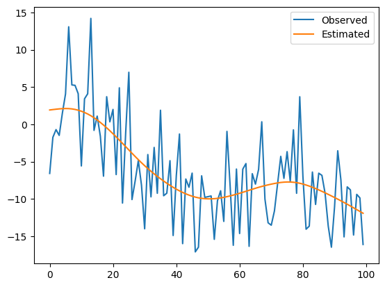
RUNNING THE L-BFGS-B CODE

           * * *

Machine precision = 2.220D-16
 N =            2     M =           10

At X0         0 variables are exactly at the bounds

At iterate    0    f=  2.60360D+00    |proj g|=  1.13647D-01

At iterate    5    f=  2.40148D+00    |proj g|=  5.58552D-03

           * * *

Tit   = total number of iterations
Tnf   = total number of function evaluations
Tnint = total number of segments explored during Cauchy searches
Skip  = number of BFGS updates skipped
Nact  = number of active bounds at final generalized Cauchy point
Projg = norm of the final projected gradient
F     = final function value

           * * *

   N    Tit     Tnf  Tnint  Skip  Nact     Projg        F
    2      8     12      1     0     0   3.529D-06   2.401D+00
  F =   2.4014289365252961     

CONVERGENCE: NORM_OF_PROJECTED_GRADIENT_<=_PGTOL            
RUNNING THE L-BFGS-B CODE

           * * *

Machine precision = 2.220D-16
 N =            3     M =           10

At X0         0 variables are exactly at the bounds

At iterate    0    f=  2.83220D+00    |proj g|=  1.08472D-01

At iterate    5    f=  2.49417D+00    |proj g|=  2.52243D-01

At iterate   10    f=  2.43783D+00    |proj g|=  2.79905D-02

At iterate   15    f=  2.41074D+00    |proj g|=  1.09463D-01

At iterate   20    f=  2.40937D+00    |proj g|=  2.39022D-06

           * * *

Tit   = total number of iterations
Tnf   = total number of function evaluations
Tnint = total number of segments explored during Cauchy searches
Skip  = number of BFGS updates skipped
Nact  = number of active bounds at final generalized Cauchy point
Projg = norm of the final projected gradient
F     = final function value

           * * *

   N    Tit     Tnf  Tnint  Skip  Nact     Projg        F
    3     20     34      1     0     0   2.390D-06   2.409D+00
  F =   2.4093731967107526     

CONVERGENCE: NORM_OF_PROJECTED_GRADIENT_<=_PGTOL            
RUNNING THE L-BFGS-B CODE

           * * *

Machine precision = 2.220D-16
 N =            3     M =           10

At X0         0 variables are exactly at the bounds

At iterate    0    f=  3.63465D+00    |proj g|=  5.67095D-02

At iterate    5    f=  2.43578D+00    |proj g|=  1.83178D-02

At iterate   10    f=  2.43362D+00    |proj g|=  4.39977D-06

           * * *

Tit   = total number of iterations
Tnf   = total number of function evaluations
Tnint = total number of segments explored during Cauchy searches
Skip  = number of BFGS updates skipped
Nact  = number of active bounds at final generalized Cauchy point
Projg = norm of the final projected gradient
F     = final function value

           * * *

   N    Tit     Tnf  Tnint  Skip  Nact     Projg        F
    3     10     19      1     0     0   4.400D-06   2.434D+00
  F =   2.4336182255825638     

CONVERGENCE: NORM_OF_PROJECTED_GRADIENT_<=_PGTOL            
                        Unobserved Components Results                         
==============================================================================
Dep. Variable:                      y   No. Observations:                  200
Model:                    local level   Log Likelihood                -480.286
Date:                Sun, 22 Sep 2024   AIC                            964.572
Time:                        13:52:11   BIC                            971.158
Sample:                             0   HQIC                           967.237
                                - 200                                         
Covariance Type:                  opg                                         
====================================================================================
                       coef    std err          z      P>|z|      [0.025      0.975]
------------------------------------------------------------------------------------
sigma2.irregular     4.2429      0.560      7.579      0.000       3.146       5.340
sigma2.level         1.2762      0.416      3.069      0.002       0.461       2.091
===================================================================================
Ljung-Box (L1) (Q):                   0.05   Jarque-Bera (JB):                 5.51
Prob(Q):                              0.83   Prob(JB):                         0.06
Heteroskedasticity (H):               1.16   Skew:                             0.40
Prob(H) (two-sided):                  0.56   Kurtosis:                         3.14
===================================================================================

Warnings:
[1] Covariance matrix calculated using the outer product of gradients (complex-step).
                        Unobserved Components Results                         
==============================================================================
Dep. Variable:                      y   No. Observations:                  200
Model:             local linear trend   Log Likelihood                -481.875
Date:                Sun, 22 Sep 2024   AIC                            969.749
Time:                        13:52:11   BIC                            979.614
Sample:                             0   HQIC                           973.742
                                - 200                                         
Covariance Type:                  opg                                         
====================================================================================
                       coef    std err          z      P>|z|      [0.025      0.975]
------------------------------------------------------------------------------------
sigma2.irregular     4.2133      0.607      6.947      0.000       3.025       5.402
sigma2.level         1.3264      0.509      2.605      0.009       0.328       2.324
sigma2.trend      2.356e-11      0.001   2.14e-08      1.000      -0.002       0.002
===================================================================================
Ljung-Box (L1) (Q):                   0.08   Jarque-Bera (JB):                 4.59
Prob(Q):                              0.78   Prob(JB):                         0.10
Heteroskedasticity (H):               1.16   Skew:                             0.36
Prob(H) (two-sided):                  0.54   Kurtosis:                         3.19
===================================================================================

Warnings:
[1] Covariance matrix calculated using the outer product of gradients (complex-step).
                           Unobserved Components Results                            
====================================================================================
Dep. Variable:                            y   No. Observations:                  200
Model:                          local level   Log Likelihood                -486.724
                   + stochastic seasonal(4)   AIC                            979.447
Date:                      Sun, 22 Sep 2024   BIC                            989.282
Time:                              13:52:11   HQIC                           983.429
Sample:                                   0                                         
                                      - 200                                         
Covariance Type:                        opg                                         
====================================================================================
                       coef    std err          z      P>|z|      [0.025      0.975]
------------------------------------------------------------------------------------
sigma2.irregular     4.6923      0.641      7.325      0.000       3.437       5.948
sigma2.level         1.3052      0.425      3.073      0.002       0.473       2.138
sigma2.seasonal   1.238e-09      0.005   2.34e-07      1.000      -0.010       0.010
===================================================================================
Ljung-Box (L1) (Q):                   0.01   Jarque-Bera (JB):                 8.08
Prob(Q):                              0.94   Prob(JB):                         0.02
Heteroskedasticity (H):               1.19   Skew:                             0.44
Prob(H) (two-sided):                  0.48   Kurtosis:                         3.47
===================================================================================

ローカルレベルモデルの推定結果をプロットします。

# プロット

plt.figure(figsize=(12, 6))

plt.plot(observed, label='Observed')

plt.plot(llm_res.level.smoothed, label='Local Level Model', linestyle=':')

plt.legend()

plt.xlabel('Time')

plt.ylabel('Value')

plt.show()

# プロット plt.figure(figsize=(12, 6)) plt.plot(observed, label='Observed') plt.plot(llm_res.level.smoothed, label='Local Level Model', linestyle=':') plt.legend() plt.xlabel('Time') plt.ylabel('Value') plt.show()

# プロット
plt.figure(figsize=(12, 6))
plt.plot(observed, label='Observed')
plt.plot(llm_res.level.smoothed, label='Local Level Model', linestyle=':')
plt.legend()
plt.xlabel('Time')
plt.ylabel('Value')
plt.show()

以下、実行結果です。

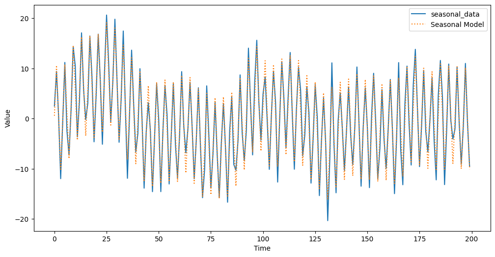
ローカルレベルモデルの推定結果をプロットします。

# プロット

plt.figure(figsize=(12, 6))

plt.plot(seasonal_data, label='seasonal_data')

plt.plot(

seasonal_res.level.smoothed + seasonal_res.seasonal.smoothed,

label='Seasonal Model', linestyle=':')

plt.legend()

plt.xlabel('Time')

plt.ylabel('Value')

plt.show()

# プロット plt.figure(figsize=(12, 6)) plt.plot(seasonal_data, label='seasonal_data') plt.plot( seasonal_res.level.smoothed + seasonal_res.seasonal.smoothed, label='Seasonal Model', linestyle=':') plt.legend() plt.xlabel('Time') plt.ylabel('Value') plt.show()

# プロット
plt.figure(figsize=(12, 6))
plt.plot(seasonal_data, label='seasonal_data')
plt.plot(
    seasonal_res.level.smoothed + seasonal_res.seasonal.smoothed, 
    label='Seasonal Model', linestyle=':')
plt.legend()
plt.xlabel('Time')
plt.ylabel('Value')
plt.show()

以下、実行結果です。

簡単な時系列データの分析例

ここでは、ローカルレベルモデルを使用して、簡単な時系列データを分析する例を示します。

import numpy as np

import pandas as pd

import statsmodels.api as sm

import matplotlib.pyplot as plt

# データの生成

np.random.seed(12345)

nobs = 200

true_state = np.cumsum(np.random.normal(size=nobs))

observed = true_state + np.random.normal(scale=0.5, size=nobs)

# モデルの定義と推定

mod = sm.tsa.UnobservedComponents(observed, 'local level')

res = mod.fit()

# 結果の表示

print(res.summary())

# フィルタリングされた状態の取得

state_estimates = res.filtered_state[0]

# プロット

plt.figure(figsize=(12,6))

plt.plot(observed, label='Observed')

plt.plot(true_state, label='True State')

plt.plot(state_estimates, label='Estimated State')

plt.legend()

plt.title('Local Level Model: True vs Estimated State')

plt.show()

import numpy as np import pandas as pd import statsmodels.api as sm import matplotlib.pyplot as plt # データの生成 np.random.seed(12345) nobs = 200 true_state = np.cumsum(np.random.normal(size=nobs)) observed = true_state + np.random.normal(scale=0.5, size=nobs) # モデルの定義と推定 mod = sm.tsa.UnobservedComponents(observed, 'local level') res = mod.fit() # 結果の表示 print(res.summary()) # フィルタリングされた状態の取得 state_estimates = res.filtered_state[0] # プロット plt.figure(figsize=(12,6)) plt.plot(observed, label='Observed') plt.plot(true_state, label='True State') plt.plot(state_estimates, label='Estimated State') plt.legend() plt.title('Local Level Model: True vs Estimated State') plt.show()

import numpy as np
import pandas as pd
import statsmodels.api as sm
import matplotlib.pyplot as plt

# データの生成
np.random.seed(12345)
nobs = 200
true_state = np.cumsum(np.random.normal(size=nobs))
observed = true_state + np.random.normal(scale=0.5, size=nobs)

# モデルの定義と推定
mod = sm.tsa.UnobservedComponents(observed, 'local level')
res = mod.fit()

# 結果の表示
print(res.summary())

# フィルタリングされた状態の取得
state_estimates = res.filtered_state[0]

# プロット
plt.figure(figsize=(12,6))
plt.plot(observed, label='Observed')
plt.plot(true_state, label='True State')
plt.plot(state_estimates, label='Estimated State')
plt.legend()
plt.title('Local Level Model: True vs Estimated State')
plt.show()

このコードは、ローカルレベルモデルを使用して、観測データから真の状態を推定します。プロットを見ることで、モデルが観測データからノイズを除去し、真の状態をどの程度正確に推定できているかを視覚的に確認することができます。

以下、実行結果です。

RUNNING THE L-BFGS-B CODE

           * * *

Machine precision = 2.220D-16
 N =            2     M =           10

At X0         0 variables are exactly at the bounds

At iterate    0    f=  2.27338D+00    |proj g|=  2.02876D-01

At iterate    5    f=  1.62080D+00    |proj g|=  5.21325D-02

At iterate   10    f=  1.61879D+00    |proj g|=  5.11060D-06

           * * *

Tit   = total number of iterations
Tnf   = total number of function evaluations
Tnint = total number of segments explored during Cauchy searches
Skip  = number of BFGS updates skipped
Nact  = number of active bounds at final generalized Cauchy point
Projg = norm of the final projected gradient
F     = final function value

           * * *

   N    Tit     Tnf  Tnint  Skip  Nact     Projg        F
    2     10     19      1     0     0   5.111D-06   1.619D+00
  F =   1.6187873637315064     

CONVERGENCE: NORM_OF_PROJECTED_GRADIENT_<=_PGTOL            
                        Unobserved Components Results                         
==============================================================================
Dep. Variable:                      y   No. Observations:                  200
Model:                    local level   Log Likelihood                -323.757
Date:                Sun, 22 Sep 2024   AIC                            651.515
Time:                        13:55:51   BIC                            658.102
Sample:                             0   HQIC                           654.181
                                - 200                                         
Covariance Type:                  opg                                         
====================================================================================
                       coef    std err          z      P>|z|      [0.025      0.975]
------------------------------------------------------------------------------------
sigma2.irregular     0.1482      0.120      1.240      0.215      -0.086       0.383
sigma2.level         1.2338      0.224      5.505      0.000       0.795       1.673
===================================================================================
Ljung-Box (L1) (Q):                   0.00   Jarque-Bera (JB):                 0.93
Prob(Q):                              0.97   Prob(JB):                         0.63
Heteroskedasticity (H):               0.88   Skew:                             0.15
Prob(H) (two-sided):                  0.61   Kurtosis:                         2.85
===================================================================================

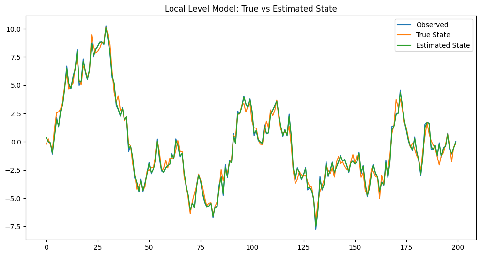
ちなみに、ここではフィルタリングの値を取得しグラフを描いています。先ほどまではスムージングの値でした。

スムージングは、フィルタリングよりも正確な推定を提供しますが、リアルタイムの予測には使用できません。

スムージング（level.smoothed）

全データを使用して、各時点での状態を最適に推定します。
過去と未来の情報を考慮して、より正確な推定を行います。

フィルタリング（filtered_state）

各時点までのデータのみを使用して状態を推定します。
リアルタイムでの推定に近く、未来の情報は考慮されません。

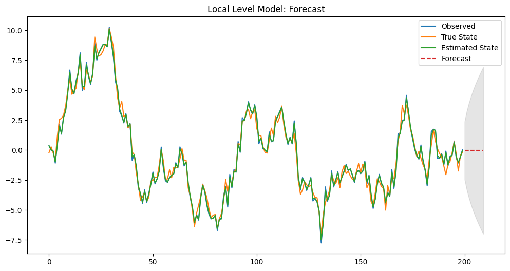
予測を行う際には、フィルタリングされた状態を使用します。予測のロジックは以下の通りです。

状態の推定: ローカルレベルモデルを使用して、観測データに基づいて状態を推定します。
フィルタリング: 各時点までのデータを使用して、状態をリアルタイムで推定します。
予測: フィルタリングされた状態を基に、将来の値を予測します。予測は、モデルが捉えたトレンドや変動を延長する形で行われます。

このプロセスにより、観測データに基づいて将来の値を予測し、その予測の信頼性を評価することができます。

以下、コード例です。

# 予測の実行

forecast = res.get_forecast(steps=10)

forecast_index = np.arange(len(observed), len(observed) + 10)

forecast_values = forecast.predicted_mean

forecast_conf_int = forecast.conf_int()

# 結果の表示

print(forecast_values)

print(forecast_conf_int)

# DataFrameに変換

forecast_conf_int_df = pd.DataFrame(forecast_conf_int)

# プロット

plt.figure(figsize=(12, 6))

plt.plot(observed, label='Observed')

plt.plot(true_state, label='True State')

plt.plot(state_estimates, label='Estimated State')

plt.plot(forecast_index, forecast_values, label='Forecast', linestyle='--')

plt.fill_between(forecast_index,

forecast_conf_int_df.iloc[:, 0],

forecast_conf_int_df.iloc[:, 1], color='gray', alpha=0.2)

plt.legend()

plt.title('Local Level Model: Forecast')

plt.show()

# 予測の実行 forecast = res.get_forecast(steps=10) forecast_index = np.arange(len(observed), len(observed) + 10) forecast_values = forecast.predicted_mean forecast_conf_int = forecast.conf_int() # 結果の表示 print(forecast_values) print(forecast_conf_int) # DataFrameに変換 forecast_conf_int_df = pd.DataFrame(forecast_conf_int) # プロット plt.figure(figsize=(12, 6)) plt.plot(observed, label='Observed') plt.plot(true_state, label='True State') plt.plot(state_estimates, label='Estimated State') plt.plot(forecast_index, forecast_values, label='Forecast', linestyle='--') plt.fill_between(forecast_index, forecast_conf_int_df.iloc[:, 0], forecast_conf_int_df.iloc[:, 1], color='gray', alpha=0.2) plt.legend() plt.title('Local Level Model: Forecast') plt.show()

# 予測の実行
forecast = res.get_forecast(steps=10)
forecast_index = np.arange(len(observed), len(observed) + 10)
forecast_values = forecast.predicted_mean
forecast_conf_int = forecast.conf_int()

# 結果の表示
print(forecast_values)
print(forecast_conf_int)

# DataFrameに変換
forecast_conf_int_df = pd.DataFrame(forecast_conf_int)

# プロット
plt.figure(figsize=(12, 6))
plt.plot(observed, label='Observed')
plt.plot(true_state, label='True State')
plt.plot(state_estimates, label='Estimated State')
plt.plot(forecast_index, forecast_values, label='Forecast', linestyle='--')
plt.fill_between(forecast_index, 
                 forecast_conf_int_df.iloc[:, 0], 
                 forecast_conf_int_df.iloc[:, 1], color='gray', alpha=0.2)
plt.legend()
plt.title('Local Level Model: Forecast')
plt.show()

以下、実行結果です。

[-0.03391005 -0.03391005 -0.03391005 -0.03391005 -0.03391005 -0.03391005
 -0.03391005 -0.03391005 -0.03391005 -0.03391005]
[[-2.44694653  2.37912642]
 [-3.28386867  3.21604856]
 [-3.94565096  3.87783086]
 [-4.51065026  4.44283016]
 [-5.01193063  4.94411053]
 [-5.46715723  5.39933712]
 [-5.88708533  5.81926522]
 [-6.27883974  6.21101963]
 [-6.64742899  6.57960888]
 [-6.99653303  6.92871292]]

Python 時系列分析 1,000本ノック– ノック69: 状態空間モデルによるフィルタリング –